Examples of Eigenproblems

A Linear Operator in the Space of Vectors on a Plane

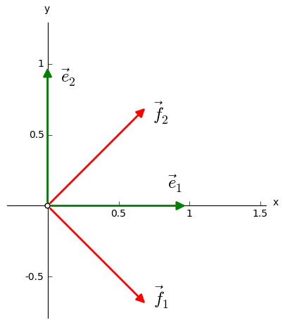
In a two-dimensional space of geometric vectors \(\,V\ \) with a basis \(\,\mathcal{B}=\{\vec{e}_1,\vec{e}_2\}\,,\ \) where \(\\\) \(\,|\vec{e}_1|=|\vec{e}_2|=1,\ \ \vec{e}_1\perp\vec{e}_2\,,\ \) we define a linear operator \(\,F\ \) by assigning the image to the vectors from the basis \(\,\mathcal{B}:\)

\[F\vec{e}_1\,=\,2\,\vec{e}_1+\vec{e}_2\,,\qquad F\vec{e}_2\,=\,\vec{e}_1+2\,\vec{e}_2\,.\]

We are looking for vectors \(\ \vec{r}\,\in\,V\!\smallsetminus\!\{\vec{0}\}\ \) which satisfy the equation \(\,F\vec{r}=\lambda\,\vec{r}\ \) for some \(\ \lambda\in R\,.\ \) When the operator \(\,F\ \) acts on these vectors it does not change their direction, but it may change their length or orientation. An outline of this situation provides a program which outputs the consecutive vectors \(\ \vec{r}\ \) from a cetain set together with their images, and emphasizes the cases when \(\ F(\vec{r})\parallel\vec{r}\ \) (after running the program, preparation of the animation takes several dozen seconds). \(\\\)

In this example we solve the eigenvalue problem for the operator \(\,F\ \) directly, without referring to the general formulae from the previous section.

By substituting \(\ \vec{r}=\alpha_1\,\vec{e}_1+\alpha_2\,\vec{e}_2\ \) to the eigenequation, we obtain:

\begin{eqnarray*} F\,\vec{r} & = & \lambda\;\vec{r}\,,\quad\vec{r}\neq\vec{0}\,, \\ F(\alpha_1\,\vec{e}_1+\alpha_2\,\vec{e}_2) & = & \lambda\;(\alpha_1\,\vec{e}_1+\alpha_2\,\vec{e}_2)\,, \\ \alpha_1\,F\vec{e}_1+\alpha_2\,F\vec{e}_2 & = & \lambda\;(\alpha_1\,\vec{e}_1+\alpha_2\,\vec{e}_2)\,, \\ \alpha_1\,(2\,\vec{e}_1+\vec{e}_2)+\alpha_2\,(\vec{e}_1+2\,\vec{e}_2) & = & \lambda\;(\alpha_1\,\vec{e}_1+\alpha_2\,\vec{e}_2)\,, \\ 2\,\alpha_1\,\vec{e}_1+\alpha_1\,\vec{e}_2+\alpha_2\,\vec{e}_1+2\,\alpha_2\,\vec{e}_2 & = & \lambda\,\alpha_1\,\vec{e}_1+\lambda\,\alpha_2\,\vec{e}_2\,, \\ \left[\,(2-\lambda)\,\alpha_1+\alpha_2\,\right]\,\vec{e}_1+\left[\,\alpha_1+(2-\lambda)\,\alpha_2\,\right]\,\vec{e}_2 & = & \vec{0}\,. \end{eqnarray*}

A linear combination of linearly independent vectors \(\ \vec{e}_1,\,\vec{e}_2\ \) from the basis \(\ \mathcal{B}\ \) equals the zero vector if and only if its coefficients do not vanish:

(1)\[\begin{split}\begin{cases}\ \ \begin{array}{c} (2-\lambda)\,\alpha_1+\alpha_2\,=\,0 \\ \alpha_1+(2-\lambda)\,\alpha_2\,=\,0 \end{array}\end{cases}\end{split}\]

The formula (1) presents a homogeneous system of two linear equations with unknowns \(\ \alpha_1,\,\alpha_2\) \(\\\) and a parameter \(\ \lambda.\ \) The non-zero solutions: \(\ \alpha_1^2+\alpha_2^2\,>\,0\,,\ \) exist if and only if

(2)\[\begin{split}\left|\begin{array}{cc} 2-\lambda & 1 \\ 1 & 2-\lambda \end{array}\right|\ =\ \lambda^2-4\,\lambda+3\ =\ (\lambda-1)(\lambda-3)\ =\ 0\,.\end{split}\]

In this way we obtained two eigenvalues of the operator \(\,F:\quad\blacktriangleright\quad\lambda_1=1\,,\ \ \lambda_2=3\,.\ \)

Substitution of \(\ \lambda=\lambda_1=1\ \) into (1) leads to an underdetermined system of equations

\[\begin{split}\quad\begin{cases}\ \begin{array}{c} \alpha_1+\alpha_2\,=\,0 \\ \alpha_1+\alpha_2\,=\,0 \end{array}\end{cases}\end{split}\]

whose solutions are of the form: \(\quad\alpha_1=\alpha\,,\ \ \alpha_2=-\;\alpha\,,\ \ \alpha\in R.\)

The eigenvectors associated with this eigenvalue:

(3)\[\blacktriangleright\quad \vec{r}_1\,=\ \alpha\,\vec{e}_1-\alpha\,\vec{e}_2\,=\ \alpha\,(\vec{e}_1-\vec{e}_2)\ \equiv\ \alpha\,\vec{f}_1\,,\quad \alpha\in R\!\smallsetminus\!\{0\}\,,\]

comprise \(\,\) (together with the zero vector \(\,\vec{0}\)) \(\,\) a 1-dimensional subspace \(\,V_1\ \) of the space \(\,V,\) \(\\\) generated by the vector \(\,\vec{f}_1=\vec{e}_1-\vec{e}_2:\) \(\ V_1=L(\vec{f}_1)\,.\)

By substituting \(\ \lambda=\lambda_2=3\ \) into \(\,\) (1) \(,\,\) we obtain the system \(\quad\begin{cases}\ \begin{array}{r} -\ \alpha_1+\alpha_2\,=\,0 \\ \alpha_1-\alpha_2\,=\,0 \end{array}\end{cases}\)

with solutions: \(\quad\alpha_1=\alpha_2=\alpha\,,\ \ \alpha\in R.\ \) The associated eigenvectors

(4)\[\blacktriangleright\quad \vec{r}_2\,=\ \alpha\,\vec{e}_1+\alpha\,\vec{e}_2\,=\ \alpha\,(\vec{e}_1+\vec{e}_2)\ \equiv\ \alpha\,\vec{f}_2\,,\quad \alpha\in R\!\smallsetminus\!\{0\}\]

also comprise \(\,\) (together with the zero vector) \(\,\) a 1-dimensional subspace, \(\\\) this time generated by the vector \(\,\vec{f}_2=\vec{e}_1+\vec{e}_2:\ \ V_2=L(\vec{f}_2)\,.\)

Note that the vectors \(\,\vec{f}_1\,,\ \vec{f}_2\ \,\) are perpendicular to each other and of the same length:

\[ \begin{align}\begin{aligned}\vec{f}_1\cdot\vec{f}_2\ =\ (\vec{e}_1-\vec{e}_2)\cdot(\vec{e}_1+\vec{e}_2)\ =\ \vec{e}_1\cdot\vec{e}_1-\vec{e}_2\cdot\vec{e}_2\ =\ |\vec{e}_1|^2-|\vec{e}_2|^2\ =\ 1-1\ =\ 0\,,\\|\,\vec{f}_{1,2}\,|^2\ =\ (\vec{e}_1\mp\vec{e}_2)^2\ =\ \vec{e}_1\cdot\vec{e}_1\mp 2\ \,\vec{e}_1\cdot\vec{e}_2+\vec{e}_2\cdot\vec{e}_2\ =\ 2\,.\end{aligned}\end{align} \]

After dividing each of the vectors \(\ \vec{f}_1,\,\vec{f}_2\ \) by its length:

(5)\[ \begin{align}\begin{aligned}\vec{f}_1\ \ \rightarrow\ \ \frac{1}{|\,\vec{f}_1\,|}\ \,\vec{f}_1\ \ =\ \ \frac{1}{\sqrt{2}}\ \,(\vec{e}_1-\vec{e}_2)\,,\\\vec{f}_2\ \ \rightarrow\ \ \frac{1}{|\,\vec{f}_2\,|}\ \,\vec{f}_2\ \ =\ \ \frac{1}{\sqrt{2}}\ \,(\vec{e}_1+\vec{e}_2)\,,\end{aligned}\end{align} \]

we obtain a pair \(\ (\vec{f}_1,\,\vec{f}_2)\ \) of unit vectors perpendicular to each other.

In this way, the space \(\,V\ \) possesses two orthonormal bases: the initial basis \(\,\mathcal{B}=(\vec{e}_1,\vec{e}_2)\ \) and the basis \(\,\mathcal{F}=(\vec{f}_1,\,\vec{f}_2)\ \) consisting of the eigenvectors of the operator \(\,F:\)

Comments and remarks.

The operator \(\,F\ \) is Hermitian because in the orthonormal basis \(\,\mathcal{B}\,\) its matrix

(6)\[\begin{split}\boldsymbol{A}\ =\ M_{\mathcal{B}}(F)\ =\ \left[\,I_{\mathcal{B}}(F\vec{e}_1)\,|\,I_{\mathcal{B}}(F\vec{e}_2)\,\right]\ =\ \left[\begin{array}{cc} 2 & 1 \\ 1 & 2 \end{array}\right]\end{split}\]

is real and symmetric, and thus Hermitian. The orthogonality of the vectors \(\ \,\vec{f}_1\ \ \text{and}\ \ \vec{f}_2\ \,\) associated to different eigenvalues, and existence of the orthonormal basis \(\ \mathcal{F}\ \,\) of the space \(\,V\ \) which comprises of the eigenvectors of the operator \(\,F\ \,\) is a consequence of this Hermitian property.

The formula (2) presents the characteristic equation of the matrix \(\,\boldsymbol{A}.\ \) Hence, and also by the formulae \(\,\) (3) \(\,\) and \(\,\) (4), \(\,\) the two eigenvalues \(\,\) \(\ \lambda_1=1\ \ \text{and}\ \ \lambda_2=3\,,\ \ \) are algebraic and of geometric multiplicty 1. The fact that the algebraic multiplicity of each eigenvalue is equal to its geometric multiplicity is also a feature of the Hermitian operators.

The basis \(\,\mathcal{F}\ \) is a result of the rotaion of the basis \(\,\mathcal{B}\ \) by the angle \(\,\pi/4.\ \) As one should expect, the change-of-basis matrix between these two orthonormal bases, determined by the formulae (5):

\[\begin{split}\boldsymbol{S}\ =\ \frac{1}{\sqrt{2}}\ \, \left[\begin{array}{rr} 1 & 1 \\ -1 & 1 \end{array}\right]\end{split}\]

is unitary (in this case: real orthogonal): \(\ \,\boldsymbol{S}^+\boldsymbol{S}=\boldsymbol{S}^{\,T}\boldsymbol{S}=\boldsymbol{I}_2\,.\)

The formula (6) presents a matrix \(\,\boldsymbol{A}\ \) of the operator \(\,F\ \) in the initial basis \(\ \mathcal{B}.\) \(\\\) Now we calculate the matrix \(\,\boldsymbol{F}=[\varphi_{ij}]\ \) of this operator in the basis \(\ \mathcal{F}\) by two methods.

• According to transformation formula for transition from the basis \(\,\mathcal{B}\ \) to \(\,\mathcal{F}:\)

  \[\begin{split}\boldsymbol{F}\ =\ \boldsymbol{S}^{-1}\boldsymbol{A}\,\boldsymbol{S}\ =\ \boldsymbol{S}^T\boldsymbol{A}\,\boldsymbol{S}\ \,=\ \, \textstyle\frac12\ \, \left[\begin{array}{rr} 1 & -1 \\ 1 & 1 \end{array}\right]\ \left[\begin{array}{cc} 2 & 1 \\ 1 & 2 \end{array}\right]\ \left[\begin{array}{rr} 1 & 1 \\ -1 & 1 \end{array}\right]\ =\ \left[\begin{array}{cc} 1 & 0 \\ 0 & 3 \end{array}\right]\,.\end{split}\]

• We get the same result by using the formulae for the matrix elements of the operator in the orthonormal basis:

  \[ \begin{align}\begin{aligned}\varphi_{11}\,=\,\boldsymbol{f}_1\cdot F\boldsymbol{f}_1\,=\, 1\ \ \boldsymbol{f}_1\cdot\boldsymbol{f}_1\,=\,1\,, \qquad \varphi_{12}\,=\,\boldsymbol{f}_1\cdot F\boldsymbol{f}_2\,=\, 3\ \ \boldsymbol{f}_1\cdot\boldsymbol{f}_2\,=\,0\,,\\\varphi_{21}\,=\,\boldsymbol{f}_2\cdot F\boldsymbol{f}_1\,=\, 1\ \ \boldsymbol{f}_2\cdot\boldsymbol{f}_1\,=\,0\,, \qquad \varphi_{22}\,=\,\boldsymbol{f}_2\cdot F\boldsymbol{f}_2\,=\, 3\ \ \boldsymbol{f}_2\cdot\boldsymbol{f}_2\,=\,3\,.\end{aligned}\end{align} \]

Matrix of the operator \(\,F\ \) in the orthonormal basis \(\ \mathcal{F}\ \) consisting of its eigenvectors is diagonal, with the eigenvalues on the diagonal.

Digression.

Each vector \(\,\vec{r}\ \) of the space \(\,V\ \) of geometric vectors on a surface may be written in a unique way as a linear combination of the basis vectors \(\,\vec{f}_1,\,\vec{f}_2:\)

\[\vec{r}\,=\,\beta_1\,\vec{f}_1+\beta_2\,\vec{f}_2\,,\qquad\beta_1,\,\beta_1\in R\,.\]

Moreover, \(\ \,\beta_1\,\vec{f}_1\in V_1\,,\ \ \beta_2\,\vec{f}_2\in V_2\,,\ \,\) where \(\ \,V_1=L(\vec{f}_1)\ \ \text{and}\ \ \,V_2=L(\vec{f}_2)\ \,\) are the subspaces of the eigenvectors of the operator \(\,F\ \) associated with the eigenvalues \(\ \lambda_1\ \ \text{and}\ \ \lambda_2,\ \,\) correspondingly. Hence, each vector \(\,\vec{r}\in V\ \) satisfies a unique decomposition

\[\vec{r}\,=\,\vec{r}_1\,+\,\vec{r}_2\,,\qquad\vec{r}_1\in V_1\,,\ \ \vec{r}_2\in V_2\,.\]

Definition.

Let \(\ V_1\,,\ \,V_2\ \,\) be subspaces of the vector space \(\,V.\ \) \(\\\) If each vector \(\,x\in V\ \) may be uniquely represented in a form \(\,x_1+x_2\,,\ \) where \(\,x_1\in V_1\ \ \text{i}\ \ x_2\in V_2\,,\ \) then we say that the space \(\,V\ \) decomposes as direct product of its subspaces \(\,V_1\ \ \text{and}\ \ V_2\,,\ \) what we write as: \(\ \ V\,=\,V_1\,\oplus\,V_2\,.\)

In our example the space \(\ V,\ \) with the action of the operator \(\,F,\ \) decomposes as direct product of the subspaces \(\ V_1\ \ \text{and}\ \ V_2\,,\ \) associated with two eigenvalues \(\ \lambda_1\ \ \text{and}\ \ \lambda_2\ \) of this operator.

Transposition of \(\ 2\times 2\ \) square matrices

We define the transposition operator \(\ T\ \) defined on the algebra \(\ M_2(R)\) \(\\\) of real square matrices of order 2:

\[\begin{split}T\ \left[\begin{array}{cc} \alpha_1 & \alpha_2 \\ \alpha_3 & \alpha_4 \end{array}\right]\ \,:\,=\ \, \left[\begin{array}{cc} \alpha_1 & \alpha_2 \\ \alpha_3 & \alpha_4 \end{array}\right]^{\,T}=\ \; \left[\begin{array}{cc} \alpha_1 & \alpha_3 \\ \alpha_2 & \alpha_4 \end{array}\right]\,,\quad \alpha_1,\,\alpha_2,\,\alpha_3,\,\alpha_4\in R\,.\end{split}\]

Because the operator \(\,T\ \) is linear and bijective, it is an automorphism of the algebra \(\,M_2(R).\)

We solve the eigenvalue problem of the operator \(\,T\ \) using the method presented in the previous section.

0.) Construction of the matrix \(\,\boldsymbol{A}=M_{\mathcal{B}}(T)\ \) of the automorphism \(\,T\ \) in a basis \(\ \mathcal{B}=(\boldsymbol{e}_1,\boldsymbol{e}_2,\boldsymbol{e}_3,\boldsymbol{e}_4)\,,\ \) where

\[\begin{split}\boldsymbol{e}_1\ =\ \left[\begin{array}{cc} 1 & 0 \\ 0 & 0 \end{array}\right]\,,\quad \boldsymbol{e}_2\ =\ \left[\begin{array}{cc} 0 & 1 \\ 0 & 0 \end{array}\right]\,,\quad \boldsymbol{e}_3\ =\ \left[\begin{array}{cc} 0 & 0 \\ 1 & 0 \end{array}\right]\,,\quad \boldsymbol{e}_4\ =\ \left[\begin{array}{cc} 0 & 0 \\ 0 & 1 \end{array}\right]\,.\end{split}\]

If we represent the images of the consecutive vectors from the basis \(\ \mathcal{B}\ \) in the same basis \(\ \mathcal{B}:\)

\begin{alignat*}{6} T\,\boldsymbol{e}_1 & {\ } = {\ \,} & \boldsymbol{e}_1 & {\ } = {\ \,} & 1\cdot\boldsymbol{e}_1 & {\ } + {\ \,} & 0\cdot\boldsymbol{e}_2 & {\ } + {\ \,} & 0\cdot\boldsymbol{e}_3 & {\ } + {\ \,} & 0\cdot\boldsymbol{e}_4\,, \\ T\,\boldsymbol{e}_2 & {\ } = {\ \,} & \boldsymbol{e}_3 & {\ } = {\ \,} & 0\cdot\boldsymbol{e}_1 & {\ } + {\ \,} & 0\cdot\boldsymbol{e}_2 & {\ } + {\ \,} & 1\cdot\boldsymbol{e}_3 & {\ } + {\ \,} & 0\cdot\boldsymbol{e}_4\,, \\ T\,\boldsymbol{e}_3 & {\ } = {\ \,} & \boldsymbol{e}_2 & {\ } = {\ \,} & 0\cdot\boldsymbol{e}_1 & {\ } + {\ \,} & 1\cdot\boldsymbol{e}_2 & {\ } + {\ \,} & 0\cdot\boldsymbol{e}_3 & {\ } + {\ \,} & 0\cdot\boldsymbol{e}_4\,, \\ T\,\boldsymbol{e}_4 & {\ } = {\ \,} & \boldsymbol{e}_4 & {\ } = {\ \,} & 0\cdot\boldsymbol{e}_1 & {\ } + {\ \,} & 0\cdot\boldsymbol{e}_2 & {\ } + {\ \,} & 0\cdot\boldsymbol{e}_3 & {\ } + {\ \,} & 1\cdot\boldsymbol{e}_4\,, \end{alignat*}

then the \(\ j\)-th column of the matrix \(\,\boldsymbol{A}\ \) comprises of the coefficients of the matrix \(\,T\boldsymbol{e}_j\,,\ \ j=1,2,3,4:\)

(7)\[\begin{split}\boldsymbol{A}\ =\ M_{\mathcal{B}}(T)\ =\ \left[\begin{array}{cccc} 1 & 0 & 0 & 0 \\ 0 & 0 & 1 & 0 \\ 0 & 1 & 0 & 0 \\ 0 & 0 & 0 & 1 \end{array}\right]\,.\end{split}\]

Now the eigenequation of the operator \(\,T:\)

\[\begin{split}T\ \left[\begin{array}{cc} \alpha_1 & \alpha_2 \\ \alpha_3 & \alpha_4 \end{array}\right]\ \,=\ \, \lambda\ \left[\begin{array}{cc} \alpha_1 & \alpha_2 \\ \alpha_3 & \alpha_4 \end{array}\right]\end{split}\]

takes the form of a homogeneous linear problem:

(8)\[\begin{split}\left[\begin{array}{cccc} 1-\lambda & 0 & 0 & 0 \\ 0 & -\ \lambda & 1 & 0 \\ 0 & 1 & -\ \lambda & 0 \\ 0 & 0 & 0 & 1-\lambda \end{array}\right]\ \left[\begin{array}{c} \alpha_1 \\ \alpha_2 \\ \alpha_3 \\ \alpha_4 \end{array}\right]\ =\ \left[\begin{array}{c} 0 \\ 0 \\ 0 \\ 0 \end{array}\right]\,.\end{split}\]

1.) Calculation of the eigenvalues as the roots of the characteristic equation.

\[\begin{split}w(\lambda)\ =\ \left|\begin{array}{cccc} 1-\lambda & 0 & 0 & 0 \\ 0 & -\ \lambda & 1 & 0 \\ 0 & 1 & -\ \lambda & 0 \\ 0 & 0 & 0 & 1-\lambda \end{array}\right|\ =\ (1-\lambda)^2\,(\lambda^2-1)\ =\ (\lambda-1)^3\,(\lambda+1)\ =\ 0\,.\end{split}\]

The eigenvalues (and their algebraic multiplicities) are then the following:

\[\blacktriangleright\qquad\lambda_1=1\quad(3)\,,\qquad\lambda_2=-1\quad(1)\,.\]

2.) Determination of eigenvectors (here: eigenmatrices).

By inserting \(\,\lambda=\lambda_1=1\ \) into the equation (8), we obtain

\[\begin{split}\left[\begin{array}{rrrr} 0 & 0 & 0 & 0 \\ 0 & -1 & 1 & 0 \\ 0 & 1 & -1 & 0 \\ 0 & 0 & 0 & 0 \end{array}\right]\ \left[\begin{array}{c} \alpha_1 \\ \alpha_2 \\ \alpha_3 \\ \alpha_4 \end{array}\right]\ =\ \left[\begin{array}{c} 0 \\ 0 \\ 0 \\ 0 \end{array}\right] ,\qquad\text{and thus}\qquad \begin{cases}\ \begin{array}{r} -\ \alpha_2+\alpha_3\,=\,0\,, \\ \alpha_2-\alpha_3\,=\,0\,. \end{array}\end{cases}\end{split}\]

The solution is of the form: \(\quad\alpha_1=\alpha\,,\ \ \alpha_2=\alpha_3=\beta\,,\ \ \alpha_4=\gamma\,,\quad \alpha,\,\beta,\,\gamma\in R.\)

The eigenmatrices of the operator \(\,T\ \) associated with the eigenvalue \(\,\lambda_1=1\,:\)

\[\begin{split}\blacktriangleright\quad \left[\begin{array}{cc} \alpha & \beta \\ \beta & \gamma \end{array}\right]\ =\ \alpha\ \left[\begin{array}{cc} 1 & 0 \\ 0 & 0 \end{array}\right]\ +\ \beta\ \left[\begin{array}{cc} 0 & 1 \\ 1 & 0 \end{array}\right]\ +\ \gamma\ \left[\begin{array}{cc} 0 & 0 \\ 0 & 1 \end{array}\right]\,,\quad \begin{array}{l} \alpha,\,\beta,\,\gamma\in R\,, \\ \alpha^2+\beta^2+\gamma^2>0 \end{array}\end{split}\]

comprise \(\,\) (after adjoining the zero matrix) \(\,\) a 3-dimensional subspace \(\ V_1\ \) of the vector space \(\ V=M_2(R),\ \\\) generated by linearly independent matrices

\[\begin{split}\boldsymbol{t}_1\ =\ \left[\begin{array}{cc} 1 & 0 \\ 0 & 0 \end{array}\right]\,,\quad \boldsymbol{t}_2\ =\ \left[\begin{array}{cc} 0 & 1 \\ 1 & 0 \end{array}\right]\,,\quad \boldsymbol{t}_3\ =\ \left[\begin{array}{cc} 0 & 0 \\ 0 & 1 \end{array}\right]\,:\qquad V_1=L(\boldsymbol{t}_1,\boldsymbol{t}_2,\boldsymbol{t}_3)\,.\end{split}\]

The eigenvalue \(\ \lambda_1=1\ \) has then both algebraic and geometric multiplicity 3.

Substitution of \(\ \lambda=\lambda_2=-1\ \) into the equation (8) gives

\[\begin{split}\left[\begin{array}{rrrr} 2 & 0 & 0 & 0 \\ 0 & 1 & 1 & 0 \\ 0 & 1 & 1 & 0 \\ 0 & 0 & 0 & 2 \end{array}\right]\ \left[\begin{array}{c} \alpha_1 \\ \alpha_2 \\ \alpha_3 \\ \alpha_4 \end{array}\right]\ =\ \left[\begin{array}{c} 0 \\ 0 \\ 0 \\ 0 \end{array}\right] ,\qquad\text{and thus}\qquad \begin{cases}\ \begin{array}{r} 2\,\alpha_1\,=\,0\,, \\ \alpha_2+\alpha_3\,=\,0\,, \\ \alpha_2+\alpha_3\,=\,0\,, \\ 2\,\alpha_4\,=\,0\,. \end{array}\end{cases}\end{split}\]

Hence \(\ \ \alpha_1=\alpha_4=0\,,\ \ \alpha_2=-\ \alpha_3=\delta\,,\ \ \delta\in R\,,\ \,\) and the eigenmatrices for the eigenvalue \(\ \lambda_2=-1:\)

\[\begin{split}\blacktriangleright\quad \left[\begin{array}{rr} 0 & \delta \\ -\delta & 0 \end{array}\right]\ =\ \delta\ \left[\begin{array}{rr} 0 & 1 \\ -1 & 0 \end{array}\right]\ =\ \delta\ \boldsymbol{t}_4\,,\qquad \boldsymbol{t}_4\,=\, \left[\begin{array}{rr} 0 & 1 \\ -1 & 0 \end{array}\right]\,,\quad \delta\in R\smallsetminus\!\{0\}\,,\end{split}\]

comprise \(\,\) (together with the zero matrix) \(\,\) a 1-dimensional subspace \(\ V_{-1}=L(\boldsymbol{t}_4)\,.\) \(\\\) The geometric multiplicity of the eigenvalue \(\ \lambda_2\ \) is the same as its algebraic multiplicity and is equal to 1.

Comments and remarks.

The eigenmatrices \(\ \boldsymbol{t}_1,\,\boldsymbol{t}_2,\,\boldsymbol{t}_3,\,\boldsymbol{t}_4\ \) are linearly independent. \(\\\) Indeed, if their linear combination is equal to the zero matrix:

\[\alpha\ \boldsymbol{t}_1\,+\,\beta\ \boldsymbol{t}_2\,+\, \gamma\ \boldsymbol{t}_3\,+\,\delta\ \boldsymbol{t}_4\ =\ \boldsymbol{0}\,,\]

then, adding the left hand side, we obtain

\[\begin{split}\left[\begin{array}{cc} \alpha & \beta+\delta \\ \beta-\delta & \gamma \end{array}\right]\ =\ \left[\begin{array}{cc} 0 & 0 \\ 0 & 0 \end{array}\right] ,\quad\text{so}\quad \begin{cases}\ \begin{array}{r} \alpha=0\,, \\ \beta+\delta=0\,, \\ \beta-\delta=0\,, \\ \gamma=0\,, \end{array}\end{cases}\quad\text{and thus}\quad \begin{cases}\ \begin{array}{r} \alpha=0\,, \\ \beta=0\,, \\ \gamma=0\,, \\ \delta=0\,. \end{array}\end{cases}\end{split}\]

The system \(\ \mathcal{T}=(\boldsymbol{t}_1,\boldsymbol{t}_2,\boldsymbol{t}_3,\boldsymbol{t}_4)\ \) is then a basis of the algebra \(\,M_2(R),\ \) an alternative for the initial basis \(\ \mathcal{B}=(\boldsymbol{e}_1,\boldsymbol{e}_2,\boldsymbol{e}_3,\boldsymbol{e}_4)\,.\ \) The connections between the vectors of these bases:

\begin{alignat*}{5} \boldsymbol{t}_1 & {\ \,} = {\ \,} & 1\cdot\boldsymbol{e}_1 {\ } + {\ } 0\cdot\boldsymbol{e}_2 {\ } + {\ } 0\cdot\boldsymbol{e}_3 {\ } + {\ } 0\cdot\boldsymbol{e}_4 \,, \\ \boldsymbol{t}_2 & {\ \,} = {\ \,} & 0\cdot\boldsymbol{e}_1 {\ } + {\ } 1\cdot\boldsymbol{e}_2 {\ } + {\ } 1\cdot\boldsymbol{e}_3 {\ } + {\ } 0\cdot\boldsymbol{e}_4 \,, \\ \boldsymbol{t}_3 & {\ \,} = {\ \,} & 0\cdot\boldsymbol{e}_1 {\ } + {\ } 0\cdot\boldsymbol{e}_2 {\ } + {\ } 0\cdot\boldsymbol{e}_3 {\ } + {\ } 1\cdot\boldsymbol{e}_4 \,, \\ \boldsymbol{t}_4 & {\ \,} = {\ \,} & 0\cdot\boldsymbol{e}_1 {\ } + {\ } 1\cdot\boldsymbol{e}_2 {\ } - {\ } 1\cdot\boldsymbol{e}_3 {\ } + {\ } 0\cdot\boldsymbol{e}_4 \,, \end{alignat*}

gives a change-of-basis matrix \(\,\boldsymbol{S}\ \) from the basis \(\,\mathcal{B}\ \) to the basis \(\,\mathcal{T}:\)

\[\begin{split}\boldsymbol{S}\ =\ \left[\begin{array}{rrrr} 1 & 0 & 0 & 0 \\ 0 & 1 & 0 & 1 \\ 0 & 1 & 0 & -1 \\ 0 & 0 & 1 & 0 \end{array}\right]\,.\end{split}\]

The formula \(\,\) (7) \(\,\) presents a matrix \(\,\boldsymbol{A}\ \) of the operator \(\,T\ \) in the initial basis \(\ \mathcal{B}.\) \(\\\) The matrix \(\ \boldsymbol{T}=[\tau_{ij}]\ \) of the operator \(\ T\ \) in the basis \(\ \mathcal{T}\ \) will be calculated by two methods.

• By definition, \(\,\) the entries \(\,\tau_{ij}\ \) of the matrix \(\,\boldsymbol{T}\ \) are defined by the equalities

  \[T\ \boldsymbol{t}_j\ =\ \tau_{1j}\ \boldsymbol{t}_1\ +\ \tau_{2j}\ \boldsymbol{t}_2\ +\ \tau_{3j}\ \boldsymbol{t}_3\ +\ \tau_{4j}\ \boldsymbol{t}_4\,,\qquad j=1,2,3,4.\]

  Taking into account that \(\,\boldsymbol{t}_i\,,\ i=1,2,3,4,\ \) are eigenmatrices of the operator \(\,T,\ \) we have:

  \begin{alignat*}{6} T\ \boldsymbol{t}_1 & {\ \,} = {\ \,} & \boldsymbol{t}_1 & {\ \,} = {\ \,} & 1\cdot\boldsymbol{t}_1 {\ } + {\ } 0\cdot\boldsymbol{t}_2 {\ } + {\ } 0\cdot\boldsymbol{t}_3 {\ } + {\ } 0\cdot\boldsymbol{t}_4 \,, \\ T\ \boldsymbol{t}_2 & {\ \,} = {\ \,} & \boldsymbol{t}_2 & {\ \,} = {\ \,} & 0\cdot\boldsymbol{t}_1 {\ } + {\ } 1\cdot\boldsymbol{t}_2 {\ } + {\ } 0\cdot\boldsymbol{t}_3 {\ } + {\ } 0\cdot\boldsymbol{t}_4 \,, \\ T\ \boldsymbol{t}_3 & {\ \,} = {\ \,} & \boldsymbol{t}_3 & {\ \,} = {\ \,} & 0\cdot\boldsymbol{t}_1 {\ } + {\ } 0\cdot\boldsymbol{t}_2 {\ } + {\ } 1\cdot\boldsymbol{t}_3 {\ } + {\ } 0\cdot\boldsymbol{t}_4 \,, \\ T\ \boldsymbol{t}_4 & {\ \,} = {\ \,} & -\ \boldsymbol{t}_4 & {\ \,} = {\ \,} & 0\cdot\boldsymbol{t}_1 {\ } + {\ } 0\cdot\boldsymbol{t}_2 {\ } + {\ } 0\cdot\boldsymbol{t}_3 {\ } - {\ } 1\cdot\boldsymbol{t}_4 \,. \end{alignat*}

  The matrix \(\,\boldsymbol{T}\ \) is then diagonal with the eigenvalues of the operator \(\,T\ \) on the diagonal:

  \[\begin{split}\boldsymbol{T}\ =\ M_{\mathcal{T}}(T)\ =\ \left[\begin{array}{rrrr} 1 & 0 & 0 & 0 \\ 0 & 1 & 0 & 0 \\ 0 & 0 & 1 & 0 \\ 0 & 0 & 0 & -1 \end{array}\right]\,.\end{split}\]
• The transformation formulae for the transition from the basis \(\ \mathcal{B}\ \) to the basis \(\ \mathcal{T}\ \) give: \(\ \ \boldsymbol{T}\ =\ \boldsymbol{S}^{-1}\boldsymbol{A}\,\boldsymbol{S}\,.\)

  In matrix calculations we use Sage:

  sage: A = matrix(QQ,[[1,0,0,0],
                       [0,0,1,0],
                       [0,1,0,0],
                       [0,0,0,1]])
  
  sage: S = matrix(QQ,[[1,0,0, 0],
                       [0,1,0, 1],
                       [0,1,0,-1],
                       [0,0,1, 0]])
  sage: S.I*A*S
  
  [ 1  0  0  0]
  [ 0  1  0  0]
  [ 0  0  1  0]
  [ 0  0  0 -1]
  

Repeating the argumentation from the previous example we can state that the space \(\ M_2(R)\ \) decomposes as direct product of subspaces \(\,V_1=L(\boldsymbol{t}_1,\boldsymbol{t}_2,\boldsymbol{t}_3)\ \) of symmetric matrices and the subspaces \(\,V_{-1}=L(\boldsymbol{t}_4)\ \) of antisymmetric matrices:

\[M_2(R)\ =\ V_1\,\oplus\,V_{-1}\,.\]