Graphical integration
Problem
Figure 1 depicts the graph of a function \(f\) defined over \(\mathbb{R}\).
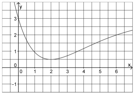
Fig. 16 Abb. 1
Determine an approximate value of \(\int\limits_3^5 f(x)\mathrm{d}x\) with the help of figure 1.
The function \(F\) is the antiderivative of \(f\) defined over \(\mathbb{R}\) with \(F(3)=0\).
Give an approximate value of the derivative of \(F\) at \(x=2\) with the help of figure 1.
Show that \(F(b) = \int\limits_3^b f(x)\mathrm{d}x\) with \(b\in\mathbb{R}\) holds.
Solution of part a
The integral corresponds to the area under the curve between the \(x\)-values 3 and 5. Thanks to the drawn grid, we can estimate the area to be about 9 squares. One square has the height and width of 0.5, respectively. The area of a square thus corresponds to 0.25, and the value of the integral is hence about 2.25.
Because the function of the graph is not explictly given, it is not easy to verify this result with Sage. However, we can try to approximately reproduce the graph with an interpolation. To this end, we choose a polynomial of degree 4 of the form
To fix the parameters \(a\) to \(e\), we have to choose five points characterizing the graph. For this purpose, we choose the points \((0|3)\), \((1|1)\), \((2|0.5)\), \((4|1.2)\) and \((6|2)\).
With the help of Sage, we can solve the corresponding linear system:
In the interval \([0, 6]\), the graph of the function agrees with the given graph quite well:
The value of the integral can be approximately reproduced as well:
Solution of part b
The derivative of the function \(F\) is the original function \(f\). Hence, we just have to read off the value of \(f\) at \(x=2\) which we have already done in part a):
The corresponding tangent line is depicted as a green line in the following part.
Solution of part c
Since \(F\) is an antiderivative of \(f\), we have
The statement to be proven follows from the supposition \(F(3)=0\).
We add \(F(x)\) to the plot of \(f\):