Application to Computer Graphics
Every 2- or 3-dimensional space can be endowed with a coordinate system at a chosen origin. In this way every object in such a space, e.g. every pixel on a computer screen, acquires coordinates which determine its position in time. Of course, at every moment of a computer game there are millions of pixels that have to be handled by a graphic card. This is possible because graphic cards may perform thousands of parallel linear computations, and - luckily - it is the compositions of linear transformations which describe many movements. Among them are rotation, scaling, shear, reflection and translation 1. We describe them and their implementation in the following sections. First try yourself if you can find a transformation which moves a single point to a desired location:
Experiment with Sage!
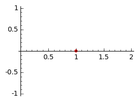
The picture on the right presents a point \(\ (1,0)\ \).
Try to find entries \(\ a, b, c, d\ \) of the matrix \(\ A\ \) in the code below which transforms this point to the point \(\ (0,1)\ \). You will see the effect on the picture which will be generated.
Can you find a matrix which sends the point \(\ (1,0)\ \) to \(\ (\frac12,0)\ \), \(\ (5,0)\ \) or \(\ (\frac{\sqrt{2}}{2},\frac{\sqrt{2}}{2})\ \)?
\(\text{}\)
2-dimensional Graphics
We start with presenting explicit forms of basic linear transformations. We will extend the idea hidden behind the exercise above to objects which are determined by a few coordinates: triangles, rectangles, circles, …
Rotation
The anti-clockwise rotation by the angle \(t\) about the origin of the coordinate system is given by the matrix
An explanation of this fact can be found in [Cam], section 5.6.3.
For example, rotation of a triangle with vertices \(\ (0, 0),\, (3, 0),\, (1,1.5)\ \) can be implemented by the following code (we marked the vertex \(\ (0, 0)\ \) for better clarity):
The first two lines are included so that you can experiment with various angles:
\(\ t\in\left[ 0, \pi/36, 2\pi/36, \ldots, 2\pi\right]\ \).
Note also that in order to access the \(i\)-th vertex of the polygon \(\ P\ \) one has to write \(\ P[0][i]\ \).
Moreover, since \(\ P[0][i]\ \) is not seen as a vector, one has to use the constructor vector() before being able to multiply it by a matrix.
Experiment with Sage!
See what happens if in the above code you replace the vertex \(\ (0, 0)\ \) of a polygon with another point, e.g. with \(\ (1, 0)\ \).
Does the triangle rotate the way you expected it?
As we said at the beginning, the rotation matrix represents the rotation about the origin. In order to rotate an object about a chosen point, one has to translate this point (and everything else) to the origin, apply the rotation matrix and translate back to the starting place.
Translation
In order to translate a point \(\ (a_1,a_2)\ \) to a point \(\ (b_1,b_2)\ \), or in other words: in order to translate a vector \(\ [a_1,a_2]\ \) to a vector \(\ [b_1,b_2]\ \), one has to add a suitable vector \(\ [t_x,t_y]\ \):
For example, if we want to shift the point \(\ (a_1,a_2)\ \) to the origin \(\ (0,0)\ \), we should shift it by the vector \(\ \left[-a_1,-a_2\right]\ \). However,
Note
Operation of addition of a fixed \(n\)-dimensional constant vector cannot be expressed by a matrix of size \(n\).
On the other hand,
In general, if we view the points in dimension greater by one (or if we write them in \(\,\) projective or homogeneous \(\,\) coordinates, see [Cam], section 6.5), then translation becomes a linear operation. This means in particular that it can be easily composed with other linear transformations. Therefore from now on all the (\(2\)-dimensional) points will have coordinates \(\ (x,y,1)\ \), and linear transformations will be given by \(\ 3\times 3\ \) matrices. In particular, the rotation matrix takes the form
and the translation by a vector \(\ [t_1,t_2]\ \) is given by
Experiment with Sage!
In order to translate a circle one only needs to know its center and radius. Run the code below and find the values of \(\ [t_1,t_2]\ \) so that the center of the circle changes from \(\ (1, 0)\ \) to \(\ (-1, 2)\ \).
Example 1.
We will rotate a triangle with vertices \(\ (1, 0),\, (3, 0),\, (1,1.5)\ \) by the angle \(t\). As before, we write the code in such a way that one can easily vary this angle.
We obtain a 3-dimensional picture because we lifted the vertices to \(\ R^3\ \). In order to present everything on a plane, we need to get rid of the last coordinate ( which will be always equal to \(1\)):
Scaling
Scaling may be done separately for each axis direction:
with respect to the \(x\)-axis: \(\ \ S_x=\left[\begin{matrix} k & 0\\ 0 & 1 \end{matrix}\right]\ \ ,\ k\in R\ \),
with respect to the \(y\)-axis: \(\ \ S_y=\left[\begin{matrix} 1 & 0\\ 0 & l \end{matrix}\right]\ \ ,\ l\in R\ \),
or in both directions at the same time, which is a result of composition of these two transformations:
Example 2.
Press Evaluate to check the effect of choice of various scales on a triangle. The original triangle is filled with light blue colour.
Experiment with Sage!
See what happens if in the code above you replace the vertex \(\ (0, 0)\ \) of the polygon \(\ P\ \) with other points, e.g. \(\ (1, 0),\, (0, 1)\ \) or \(\ (2, 2)\ \).
How does the coordinate which is equal to zero influence the result?
The reason for the above phenomenon is that scaling scales the whole axis, not just the object. Therefore, as it was the case with rotation, if one wants to scale an object and keep one of the vertices at the same place, one has to translate the chosen vertex to the origin, apply scaling and translate everything back.
Now that we need to use translation, we go back to homogeneous coordinates. In particular, the scaling matrix takes the form
It is easy to see that in general scaling changes the volume and shape of an object. The only case when volume is preserved is when the scales \(\ k,l\ \) satisfy \(\ k=\frac1l\ \) (this defines a squeeze mapping \(\,\)). The shape is preserved if and only if \(\ k=l\ \). Try some of such values in the code above!
Shear
As it was the case for scaling, we distinguish two types of shearing mappings:
horizontal shear (parallel to the \(x\)-axis): \(\ \ Sh_x=\left[\begin{matrix} 1 & a\\ 0 & 1 \end{matrix}\right]\ ,\ a\in R\ \),
vertical shear (parallel to the \(y\)-axis): \(\ \ Sh_y=\left[\begin{matrix} 1 & 0\\ b & 1 \end{matrix}\right]\ ,\ b\in R\ \).
Observe their effect by running the code below and changing the values of parameters \(\ a\ \) and \(\ b\ \). Start with setting one of them to be equal to zero.
As you could see, varying \(\ a\ \) ( which is responsible for shear parallel to the \(x\)-axis) resulted in shifting the parallelogram away from the \(y\)-axis. As you might have guessed by now, the reason is that none of \(y\)-coordinates of the parallelogram is equal to zero. Indeed, for a point \(\ p=(x_p,y_p)\ \):
which means that for any \(\ a\neq 0\ \), \(\ x_p+a y_p\neq x_p\ \) whenever \(\ y_p\neq 0\ \), that is: if \(\ y_p\neq 0\ \), then the \(x\)-coordinate of the point \(\ p\ \) will always change.
In order to produce the shear effect and keep it attached to the chosen vertex, we have to move to projective coordinates and apply the translation trick. In this setting shear matrices are of the form
Exercise.
Produce the shear effect with parameters \(\ a = 3,\, b=0\ \) for the parallelogram from the code above so that the resulting parallelogram remains attached to the vertex \(\ (0,1)\ \). Write suitable code in the window below.
Reflection
In order to find reflection of the point \(\ p\ \) with respect to the line \(\ l\ \), one has to construct the line \(\ l'\ \) which is orthogonal to \(\ l\ \) and passes throught the point \(\ p\ \), and then mark the point on \(\ l'\ \) whose distance from \(\ l\ \) is the same as distance of \(\ p\ \) from \(\ l\ \).
If we want to find a reflection with respect to the \(y\)-axis, that is \(\ l:\ x=0\ \), then the reflection \(\ q\ \) of the point \(\ p=(x_p,y_p)\ \) has coordinates \(\ q=(-x_p,y_p)\ \), e.g.
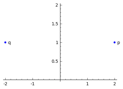
This corresponds to a linear transformation given by matrix \(\ R_{\infty}=\left[\begin{matrix} -1 & 0 \\ 0 & 1\end{matrix}\right]\ \) as
In general, reflection \(\ q\ \) of the point \(\ p=(x_p,y_p)\ \) with respect to the line passing through the origin: \(\ l:\ y=ax\, ,\, a\in R\ \) is given by the formula \(\ q=((-1+\frac{2}{1+a^2})x_p+ \frac{2a}{1+a^2} y_p, \frac{2a}{1+a^2} x_p+(1-\frac{2}{1+a^2})y_p)\ \), which is described by the matrix
Example 3.
The following code describes reflection of a triangle with respect to a line \(\ l:\ y=ax\, ,\, a\in [-5,5]\ \). Observe that again it suffices to determine the action on the vertices of the triangle. Press Evaluate to observe the effect for various values of \(\ a\ \). How does the picture change when \(\ a\ \) increases or decreases? How is this related to reflection defined by \(\ R_{\infty}\ \)?
Projection
We distinguish projections to the \(x\)-axis and to the \(y\)-axis:
Projection to the \(x\)-axis. \(\ \qquad\qquad\ \) Projection to the \(y\)-axis.
They are given by projection matrices which neglect the input of the \(y\)- or \(x\)-coordinate, correspondingly:
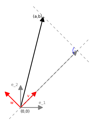
These projections are very natural, because we often choose the coordinate system whose axes agree with the standard (orthogonal) basis vectors: \(x\)-axis with \(\ e_1=[1,0]\ \) and \(y\)-axis with \(\ e_2=[0,1]\ \). In this way every point \(\ (a,b)\ \) on a plane determines a vector \(\ [a,b]=ae_1+be_2\ \). If we project to the \(x\)-axis, then since the vectors \(\ e_1\ \) and \(\ e_2\ \) are orthogonal, the contribution from the second vector vanishes (for more details look at the chapter Unitary Spaces). However, if we change the basis from \(\ e_1,\, e_2\ \) to an (orthonormal) basis \(\ v,\, w\ \) 2, then it is equaly easy to find \(\ \alpha ,\,\beta\ \) so that \(\ [a,b]=\alpha v+\beta w\ \). Then the projection of the point \(\ (a,b)\ \) to the axis determined by the vector \(\ v\ \) will be equal to \(\ \alpha\ \). In fact, we know the precise formulae for \(\ \alpha\ \) (see Example 4). in Inner (Scalar) Product), which allows us to give a matrix representation of projection onto the vector \(\ v=[v_1,v_2]\ \):
if \(v\) is not of length \(1\), one has to normalise the matrix by dividing each entry by \(\ v_1^2\, +\,v_2^2\ \).
Example 4
Press Evaluate to observe the effect of projecting the figure from example above onto various vectors \(v\). The code also returns coordinates of a vector and projection matrix that were used.
Functional programming
In this section we briefly introduce a concise way of transforming big lists of points at the same time. We limit ourselves to one example; the interested reader will find a more detailed treatment of this topic at
http://doc.sagemath.org/html/en/thematic_tutorials/functional_programming.html .
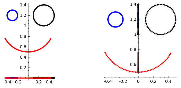
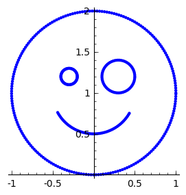
Consider a picture given by a set of points defined by the following code:
sage: pic=[vector([cos(x),1+sin(x)]) for x in srange(0,2*pi,0.03)]
sage: pic+=[vector([0.3+.2*cos(x),1+0.2+.2*sin(x)]) for x in srange(0,2*pi,0.1)]
sage: pic+=[vector([-0.3+.1*cos(x),1+0.2+.1*sin(x)]) for x in srange(0,2*pi,0.1)]
sage: pic+=[vector([.5*cos(x),1+.5*sin(x)]) for x in srange(pi+.5,2*pi-.5,0.04)]
sage: points(pic).show(aspect_ratio=1,figsize=4) # points() transforms a list of pairs to a set of points
In order to apply a linear transformation to such a big set we could proceed as previously,
that is, to create long lists of points and use a loop to apply an action of the
matrix on each of the points. This may be written in a cleaner way by
applying the Python built-in function map(), which applies one
function (provided as the first argument) to each element of the chosen
domain (provided as the consecutive arguments). In our case, the function takes one argument
and multiplies it by a fixed matrix \(\ A\ \);
such function may be defined shortly using lambda statement as below.
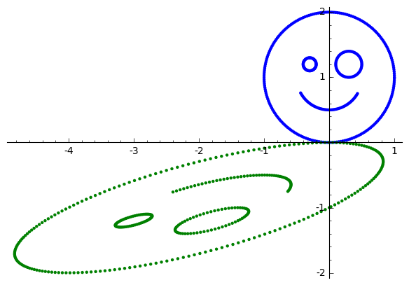
For example, to transform the above picture by the matrix
\(\ A=\left[\begin{matrix} 2 & -2 \\ 0 & -1 \end{matrix}\right]\ \), we write:
sage: A=matrix([[2,-2],[0,-1]])
sage: Apic=map(lambda w: A*w,pic)
# lambda w: A*w defines a function "multiply w by A on the left"
# second argument pic provides a set on which this function is defined
sage: newpic=points(pic)+points(Apic,color='green')
sage: newpic.show(aspect_ratio=1,figsize=(6,6))
Experiment with Sage!
The code below transforms the picture introduced above by a randomly chosen \(\ 2\times 2\ \) matrix. Can you find a decomposition of this matrix to linear transformations that were introduced above?
In order to transform a colorful picture and preserve the colour under every transformation, one may create a list which stores information on colours in RGB format (with values between \(0\) and \(1\)) and assign them to points/figures/etc. in a desirable manner. This was done on a small scale in Example 4. above. To introduce more complicated colouring (and with use of lambda and map()) one can proceed as follows:
Note that Apic which is defined via map(lambda w: A*w,pic) is a list of vectors A*w, where w runs over the consecutive elements of the list pic. Therefore the order of colouring of the initial points and the points after multiplication by A will be the same.
Experiment with Sage!
Change the code above so that the eyes of the figure are all blue and they remain blue after a transformation.
Modelling of movement
We finish discussion on fundamentals of 2d graphics with an example of modelling of movement of a simple object along a given curve.
Example 5.
If we ignore air resistance, then position of a ball shot from the cannon with velocity \(\ v_0\ \) at an angle of \(\ \alpha\ \) degrees is described by the equation
where \(\ g=9.80665 \frac{m}{s^2}\ \) denotes standard gravity and the coordinate system is chosen so that the cannon is placed at the origin. In order to model the movement of this ball it suffices to know the position of its centre, which at the \(i\)-th moment will be denoted by \(\ (x_i,y_i)\ \). The consecutive positions of the centre may be viewed as an effect of its translations along the curve \(\ f(x)=x\tan\alpha -\frac{g}{2v_0^2\cos^2\alpha}x^2\ \), that is (in projective coordinates),
for some \(\ a,\, b>0\ \). From here we see that
After the time \(\ t\ \), the ball covers the horizontal distance (i.e. along the \(x\)-axis) described by \(\ x(t)=v_0t\cos\alpha\ \). Hence, if \(\ i\ \) describes the unit of time, then \(\ a=x_{i+1}-x_i=v_0\cos\alpha\ \) and
If we let \(\ A=-\frac{g}{a}\ \), \(\ B=a\tan\alpha-\frac{g}{2}\ \), then the translation matrix takes the form
The above considerations can be implemented in Sage as follows:
Experiment with Sage!
Change the values of the initial velocity v0 and the angle al
in the code above to observe how these values affect the range of movement and the
time before the ball hits the ground.
Observe how the distance covered within the same amount of time (gaps between the consecutive dots on the picture)
varies depending on the position of the ball.
Now it is very easy to adjust the code written above to produce an animation:
Note that at the second to the last line we fixed the minimal and maximal points on the \(x\)- and \(y\)-axes. Thanks to this the axes stay fixed during the animation.
Experiment with Sage!
Produce an animation for various values of v0 and the angle al (the greater v0, the longer the animation).
To obtain more refined movement, shorten the time unit in which the position of the ball is computed:
replace t=1 and t=t+1 with t=0.5 and t=t+0.5 or with smaller values.
In a similar way we can adjust previously created code to produce an animation:
1). Create a list which stores the points that define an object.
2). Define a number of frames for an animation (the range).
3). Animate an object (provide bounds for the axes).
Example 6.
The code below generates a rotating triangle. Observe minor changes that had to be applied to the code from Example 1.
sage: L=list()
sage: t=0
sage: for j in range(72):
sage:     R=Matrix([[cos(t),-sin(t),0],[sin(t),cos(t),0],[0,0,1]])
sage:     P=polygon2d([(1, 0), (3, 0), (1,1.5)])
sage:     Pl=[list(P[0][i])+[1] for i in range(3)]
sage:     tr=[-P[0][0][i] for i in range(2)]
sage:     T=Matrix([[1,0,tr[0]],[0,1,tr[1]],[0,0,1]])
sage:     V=list(T.inverse()*R*T*vector(Pl[i]) for i in range(3))
sage:     L.insert(j,[(V[i][0],V[i][1]) for i in range(3)])
sage:     t=t+pi/36
sage: rotatetriangle=animate([polygon(L[t]) for t in range (72)], xmin=-3, xmax=3, ymin=-3, ymax=3)
sage: rotatetriangle.show()
Exercises
The exercises can be downloaded in a form of a notebook from here .
Exercise 1.
Define a polygon on vertices \(\ (3,3),\, (2,3+\sqrt{3}),\, (3,3+\frac{2\sqrt{3}}{3}),\, (4,3+\sqrt{3})\ \) and find its reflection with respect to a line \(\ l: y=2x-1\ \).
(Hint: Use the translation with t_1=0, t_2=1.)
Exercise 2.
Produce an animation which rotates the polygon from Exercise 1.
a). around the origin \(\ (0,0)\ \),
b). around the point \(\ (3,3)\ \).
c). Fill in the code below to produce the following effect (each part should be done in a separate window; the commands written at the bottom verify whether the third vertex of the polygon is translated to a correct position):
first \(\ 60^{\circ}\ \) of rotation is around the point \(\ (3,3)\ \),
- next \(\ 120^{\circ}\ \) of rotation is around the point \(\ (1,3)\ \)
(this is where the vertex \(\ (2,3+\sqrt{3})\ \) lands after rotation by \(\ 60^{\circ}\ \)),
next \(\ 120^{\circ}\ \) of rotation is around the point \(\ (-1,3)\ \),
last \(\ 60^{\circ}\ \) of rotation is around the point \(\ (-3,3)\ \).
d). Use the code produced in point c). to obtain an animation.
e). Mark a thick red point on the vertex \(\ (3,3)\ \). Imagine that this is a ball which rolls along the edge of the polygon while the polygon is rotating. Include the movement of this ball inside the polygon.
- 1
As we explain in the subsequent part of this section, translation of a 2-dimensional object becomes a linear transformation when it is viewed in a 3-dimensional space (but not 2-dimensional!).
- 2
The basis \(\ \left\{ \left[v_1,v_2\right],\, \left[w_1,w_2\right]\right\}\ \) is orthonormal if the basis vectors are orthogonal (perpendicular) and are of length \(1\), that is, \(\ v_1w_1+v_2w_2=0\ \) and \(\ v_1^2+v_2^2=1\ \), \(\ w_1^2+w_2^2=1\ \). (For details consult chapter Unitary Spaces.)
- Cam(1,2)
Jonathan G. Campbell, Notes on Mathematics for 2D and 3D Graphics. Available at http://www.multiresolutions.com/strule/jon/www-jgcampbell-com/bscgp1/grmaths.pdf