Geometry of Linear Equations

In this section we shall discuss systems of linear equations in two or three variables over the real field \(\,R.\,\) Such systems can be directly visualized, either in a plane by a set of straight lines, or in the three-dimensional (still imaginable) space by a collection of planes.

We shall focus on two geometric approaches to linear systems: the row picture and the column picture. This terminology concerns rows and columns of the coefficient matrix which, together with the vector of constants, represents a system of equations. We also mention the algebraic matrix picture, which is the starting point for the general theory, developed in next chapters.

The intended purpose of simple examples shown here is (hopefully) to expand the intuition, useful for dealing with greater linear systems represented by sets of hyperplanes in multi-dimensional spaces.

Row Picture

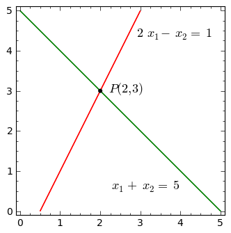
Consider the following system of two linear equations:

\begin{alignat*}{3} 2\,x_1 & {\,} - {\,} & x_2 & {\;} = {\;} & 1 \\ x_1 & {\,} + {\,}& x_2 & {\;} = {\;} & 5 \end{alignat*}

It may be solved by hand or by computer:

to yield the solution \(\ x_1=2,\ x_2=3.\)

Each equation is represented by a straight line in the plane \((x_1,x_2).\) The solution corresponds to a point lying on both lines simultaneously, that is to the point of intersection of these lines:

In general, two straight lines in a plane may behave in three ways:

1. \(\,\) lines intersect at a single point;

2. \(\,\) lines are identical and merge together;

3. \(\,\) lines are parallel (though different).

Accordingly, a corresponding system of two equations:

1. \(\,\) has a single unique solution;

2. \(\,\) has infinitely many solutions;

3. \(\,\) has no solution.

When a system of equations has at least one solution (case 1. and 2. above), \(\\\) it is said to be \(\,\) consistent, \(\,\) otherwise (case 3.) it is \(\,\) inconsistent. \(\\\) On the other hand, a system with more than one solution (case 2.) is \(\,\) indeterminate.

Column Picture

The foregoing system of equations

\begin{alignat*}{3} 2\,x_1 & {\,} - {\,} & x_2 & {\;} = {\;} & 1 \\ x_1 & {\,} + {\,}& x_2 & {\;} = {\;} & 5 \end{alignat*}

can be rewritten as equality of two column vectors:

\[\begin{split}\left[\begin{array}{r} 2\,x_1\ -\ x_2 \\ x_1\ +\ x_2 \end{array}\right] \ =\ \left[\begin{array}{c} 1 \\ 5 \end{array}\right]\,.\end{split}\]

The left-hand side can be expressed as a linear combination with coefficients \(\,x_1,\,x_2\,:\)

\[\begin{split}x_1\ \left[\begin{array}{r} 2 \\ 1 \end{array}\right] \ + \ x_2\ \left[\begin{array}{r} -1 \\ 1 \end{array}\right] \ = \ \left[\begin{array}{r} 1 \\ 5 \end{array}\right]\,.\end{split}\]

Now the unknowns \(\,x_1,\,x_2\ \) are weights for column vectors \(\ \boldsymbol{a}_1 = \left[\begin{array}{r} 2 \\ 1 \end{array}\right],\ \) \(\boldsymbol{a}_2 = \left[\begin{array}{r} -1 \\ 1 \end{array}\right]\ \) \(\\\) in a linear combination, \(\,\) which should equal the column vector of constants \(\ \boldsymbol{b}\,= \left[ \begin{array}{r} 1 \\5 \end{array} \right].\)

Experiment with Sage:

In the following program the column vectors \(\;\boldsymbol{a}_1,\ \boldsymbol{a}_2\ \) and \(\;\boldsymbol{b}\ \) are represented by the geometric vectors \(\;\vec{a}_1,\ \vec{a}_2\ \) and \(\;\vec{b},\ \) respectively. Using the sliders, set the values of coefficients \(\ x_1\ \) and \(\ x_2\ \) so that the vector \(\;x_1\ \vec{a}_1 + x_2\ \vec{a}_2\;\) (coloured grey) is equal to the vector \(\,\vec{b}\).

In general, a system of linear equations is completely determined by the coefficient matrix \(\,\boldsymbol{A}\ \) and the vector of constants \(\,\boldsymbol{b}.\ \) In the present example

\[\begin{split}\boldsymbol{A}\ = \ \left[\begin{array}{rr} 2 & -1 \\ 1 & 1 \end{array}\right]\,,\qquad \boldsymbol{b}\ =\ \left[\begin{array}{c} 1 \\ 5 \end{array}\right]\,.\end{split}\]

The row picture of a system of equations is obtained by reading the rows of matrix \(\,\boldsymbol{A},\ \) whereas the column picture involves the columns thereof.

\(\ \)

Consistent System: a unique solution

We shall deal with the system of three equations in three variables:

\begin{alignat*}{4} 2\,x_1 & {\,} + {\,} & x_2 & {\,} + {\,} & x_3 & {\;} = {} & 1 \\ x_1 & {\,} - {\,} & x_2 & & & {\;} = {} & -1 \\ x_1 & {\,} + {\,} & x_2 & {\,} + {\,} & 2\,x_3 & {\;} = {} & 2 \end{alignat*}

Its solution is given by \(\ \ x_1 = -\frac{1}{4},\ \ x_2 = \frac{3}{4},\ \ x_3 = \frac{3}{4}\,.\)

In the three-dimensional space of coordinates \(\ x_1,\,x_2,\,x_3\ \) each linear equation yields a plane. In the row picture, the solution of the system is therefore given by the geometric locus of points belonging simultaneously to the three planes. In the present case, this is the single point of their intersection.

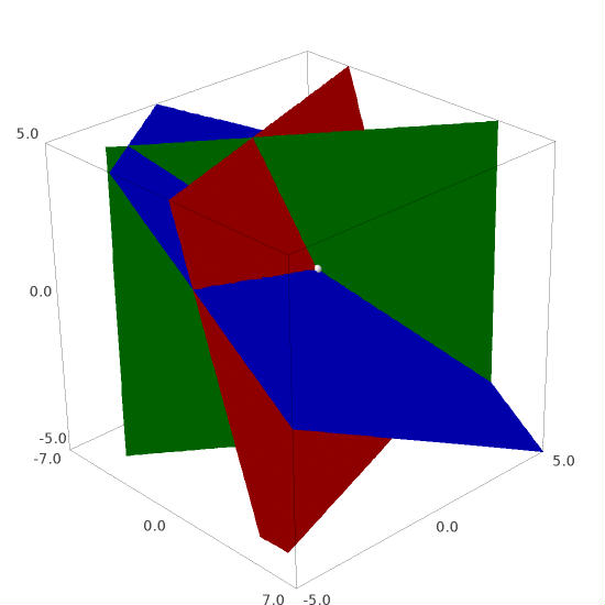
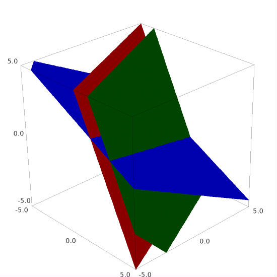
Row picture. The planes corresponding to the consecutive equations of the system are coloured red, green and blue, respectively, whereas the point common to them (representing the solution) is drawn in white.

In the column picture the problem consists in determining the coefficients \(\ x_1,\,x_2,\,x_3\ \,\) \(\\\) in a linear combination of column vectors \(\ \boldsymbol{a}_1,\,\boldsymbol{a}_2,\,\boldsymbol{a}_3\,,\ \) which is equal to vector \(\,\boldsymbol{b}:\)

(1)\[x_1\,\boldsymbol{a}_1\,+\,x_2\,\boldsymbol{a}_2\,+\,x_3\,\boldsymbol{a}_3\ = \ \boldsymbol{b}\,.\]

The function verse3column() writes down a given system of three linear equations in three unknowns in the column form (1):

The function has to be called with a list of equations as the argument:

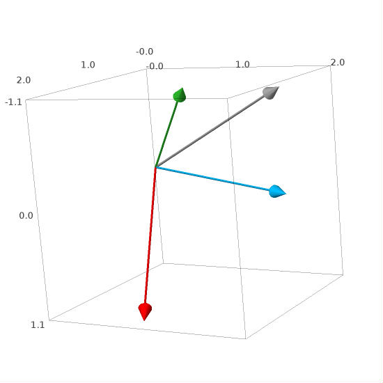
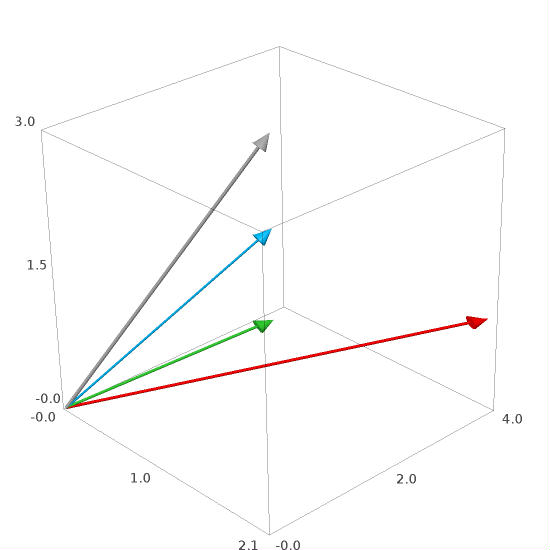
Column picture. The vectors \(\ \boldsymbol{a}_1,\,\boldsymbol{a}_2,\,\boldsymbol{a}_3\ \) and \(\ \boldsymbol{b}\ \) are coloured red, green, blue and grey, respectively. The uniqueness of the solution stems from the fact that \(\ \boldsymbol{a}_1,\,\boldsymbol{a}_2,\,\boldsymbol{a}_3\ \) are not coplanar, thereby creating a basis in the three-dimensional space of geometric vectors.

Consistent System: infinitely many solutions

Now we shall discuss the following system of linear equations:

\begin{alignat*}{4} 2\,x_1 & {\,} + {\,} & x_2 & {\,} + {\,} & x_3 & {\;} = {\;} & 1 \\ 4\,x_1 & {\,} + {\,} & 2\,x_2 & {\,} + {\,} & 2\,x_3 & {\;} = {\;} & 2 \\ x_1 & {\,} + {\,} & x_2 & {\,} + {\,} & 2\,x_3 & {\;} = {\;} & 3 \end{alignat*}

The Sage function solve() yields the solution dependent on a parameter \(\,r_1,\,\) which may assume arbitrary values:

Therefore, the equations are simultaneously satisfied with infinitely many triplets of numbers.

This outcome is a consequence of a linear dependence of equations. In general, a system of linear equations is said to be (linearly) dependent, when one of the equations can be expressed as a linear combination of the remaining ones, that is when one equation can be algebraically derived from the others. Such equation does not contribute any new information about variables and removing it does not change the set of solutions.

In the present example, the second equation is simply the first one scaled by a factor of two. Thus actually we have to deal with a system of two (independent) equations in three variables.

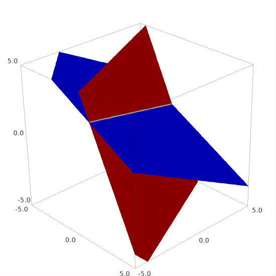
Row picture. The planes, corresponding to the two first equations (coloured red and green) are identical and merge together. The blue plane, corresponding to the third equation, intersects them along the (white) straight line. That line represents the infinite set of solutions of the system.

Column picture. The vectors \(\ \vec{a}_1,\,\vec{a}_2,\,\vec{a}_3\ \) (coloured red, green, blue, respectively) are coplanar. The vector \(\ \vec{b}\,\) (grey), representing the vector of constants, belongs to the same plane. In this situation infinitely many linear combinations of vectors \(\ \vec{a}_1,\,\vec{a}_2,\,\vec{a}_3\ \) may be equal to \(\ \vec{b}.\)

A remark on indeterminate systems of equations.

Suppose that solving a system of equations (not necessarily linear) with the aid of the Sage function solve() resulted in expressions containing parameters \(\ \) r1, r2, ... \(\\\) (their names are unpredictable). If we want to make use of these parameters for, say, drawing solutions, then before using them we have to declare the corresponding variables.

In the present example we consider a trivial indeterminate system of two linear equations in two variables, whose solution depends on a single parameter. The following procedure makes it possible to draw the set of solutions for a given range of the parameter.

We encourage the reader to analyze the code and to become acquainted with the advanced tools of Sage applied herein.

Inconsistent System: no solution

We shall slightly modify the previous example by changing its right-hand side:

\begin{alignat*}{4} 2\,x_1 & {\,} + {\,} & x_2 & {\,} + {\,} & x_3 & {\;} = {\;} & 0 \\ 4\,x_1 & {\,} + {\,} & 2\,x_2 & {\,} + {\,} & 2\,x_3 & {\;} = {\;} & 5 \\ x_1 & {\,} + {\,} & x_2 & {\,} + {\,} & 2\,x_3 & {\;} = {\;} & 1 \end{alignat*}

Now the system no longer has any solution:

Indeed, there is an obvious contradiction between the first two equations. The left-hand side of the second equation being the double of the left-hand side of the first one, the right-hand side of the second equation should equal 0, not 5.

Below we study a graphical representation of this situation, using the row and column pictures of a linear system.

Row picture. \(\\\) The planes, corresponding to the first two equations of the system (coloured red and green) are parallel, but do not merge. Thus regardless of a position of the third (blue) plane, representing the third equation, the geometric locus of points common to all three planes is the empty set. \(\\\) \(\\\)

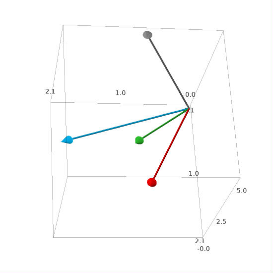
Column picture. \(\,\) As previously, the vectors \(\,\vec{a}_1,\,\vec{a}_2,\,\vec{a}_3\,\) (red, green, blue) are coplanar. \(\\\) In contrast to the previous case however, vector \(\ \vec{b}\,\) (grey) is not coplanar with them. None of the linear combinations of \(\ \vec{a}_1,\,\vec{a}_2,\,\vec{a}_3\ \) can equal \(\ \vec{b},\ \) hence the set of solutions is empty.

Matrix Picture of a Linear System

Let’s reconsider the generic system of three equations in three variables:

\begin{alignat*}{4} 2\,x_1 & {\,} + {\,} & x_2 & {\,} + {\,} & x_3 & {\;} = {} & 1 \\ x_1 & {\,} - {\,} & x_2 & & & {\;} = {} & -1 \\ x_1 & {\,} + {\,} & x_2 & {\,} + {\,} & 2\,x_3 & {\;} = {} & 2 \end{alignat*}

where the matrix of coefficients and the vector of constants are given by

\[\begin{split}\boldsymbol{A}\ =\ \left[\,\boldsymbol{a}_1\,|\,\boldsymbol{a}_2\,|\,\boldsymbol{a}_3\,\right] \ =\ \left[\begin{array}{rrr} 2 & 1 & 1 \\ 1 & -1 & 0 \\ 1 & 1 & 2 \end{array}\right]\,,\qquad \boldsymbol{b}\ =\ \left[\begin{array}{r} 1 \\ -1 \\ 2 \end{array}\right]\,.\end{split}\]

A product of the matrix \(\,\boldsymbol{A}\ \) and the column vector \(\,\boldsymbol{x}\ \) of unknowns being defined as

\[\begin{split}\boldsymbol{A}\,\boldsymbol{x}\ \equiv\ \left[\,\boldsymbol{a}_1\,|\,\boldsymbol{a}_2\,|\,\boldsymbol{a}_3\,\right]\ \left[\begin{array}{r} x_1 \\ x_2 \\ x_3 \end{array}\right]\ \ :\,=\ \ x_1\ \boldsymbol{a}_1\ +\ x_2\ \boldsymbol{a}_2\ +\ x_3\ \boldsymbol{a}_3\,,\end{split}\]

the column form of the above system

\[\begin{split}x_1\ \left[\begin{array}{r} 2 \\ 1 \\ 1 \end{array}\right]\ +\ \, x_2\ \left[\begin{array}{r} 1 \\ -1 \\ 1 \end{array}\right]\ +\ \, x_3\ \left[\begin{array}{r} 1 \\ 0 \\ 2 \end{array}\right] \ =\ \left[\begin{array}{r} 1 \\ -1 \\ 2 \end{array}\right]\,,\end{split}\]

can be rewritten in a compact matrix form as \(\ \ \boldsymbol{A} \boldsymbol{x} = \boldsymbol{b}\,.\) \(\\\) The latter formula may be called \(\,\) a \(\,\) matrix picture \(\,\) of a linear system.