Properties of the square root function

Problem 1

Given the function \(f:x\mapsto 2-\sqrt{12-2x}\) with a maximal domain \(\mathbb{D}_f=]-\infty;6]\), we denote the graph of \(f\) by \(G_f\).

1. Calculate the coordinates of the intersection points of \(G_f\) and the coordinate axes. Determine the behavior of \(f\) in the limit \(x\rightarrow-\infty\) and calculate \(f(6)\).

2. Determine the derivative \(f'\) of \(f\) and indicate the maximal domain for \(f'\). Determine \(\lim\limits_{x\rightarrow6}f'(x)\). Which property arises from this result?

3. Describe the monotonic behavior of \(G_f\) and state the codomain of \(f\).

4. Determine \(f(-2)\) and draw \(G_f\) in a coordinate system taking into account the previous results. (Space needed in view of the following tasks: \(-3\leq y\leq 7\)).

5. The function \(f\) can be inverted in \(\mathbb{D}_f\). Give the domain for the inverse function \(f^{-1}\) of \(f\) and prove that \(f^{-1}(x)=-\frac{1}{2}x^2+2x+4\).

Solution of part 1a

First, we make use of Sage to obtain an overview of the given function.

The intersection of \(f\) and the \(y\)-axis is located at \((0|f(0))\) with

\[f(0)=2-2\sqrt{3}.\]

This can be checked using Sage:

The intersection of \(f\) and the \(x\)-axis is given by the zero of the function \(f\):

\[f(x) = 2-\sqrt{12-2x} \overset{!}{=} 0\]

Solving the equation for \(x\) leads to

\[x=4,\]

which is confirmed by Sage:

Thus, we obtain exactly one intersection of \(f\) and the \(x\)-axis located at \((4|0)\).

The two intersections with the coordinate axes are consistent with the graph of \(f\) obtained earlier by means of Sage.

For the behavior of \(f(x)\) in the limit \(x\rightarrow -\infty\), we find

\[\begin{split}\lim\limits_{x\rightarrow -\infty} 2-\sqrt{12-2x} &= \lim\limits_{x\rightarrow \infty} 2-\sqrt{12+2x}\\ &= -\lim\limits_{x\rightarrow \infty} \sqrt{2x}\\ &= -\infty.\end{split}\]

This can be verified with Sage:

The value \(f(6)\) can be determined as

\[f(6) = 2-\sqrt{12-2\cdot6}=2.\]

This result can also be obtained from the graph of the function.

Solution of part 1b

The derivative of \(f\) can be calculated by using the chain rule:

\[f'(x) = -\frac{1}{2} (12-2x)^{-\frac{1}{2}}\cdot(-2) = \frac{1}{\sqrt{12-2x}}.\]

The same result is obtained by means of Sage:

Compared to the domain of \(f\), the domain of the derivative is obtained by taking out the zero of the denominator at \(x_0=6\), i.e. \(\mathbb{D}_{f'}=]-\infty;6[\).

The limit \(\lim\limits_{x\rightarrow 6}f'(x)\) can be calculated as

\[\lim\limits_{x\rightarrow 6}f'(x) = \lim\limits_{x\rightarrow 0}\frac{1}{\sqrt{x}}=\infty,\]

This result can read off the graph of \(f'(x)\) or determined by means of Sage:

Solution of part 1c

In order to determine the monotonic behavior of \(f\), we have to analyze its derivative \(f'\). From the graph of \(f'\) we conclude that \(f'\) is positive in every point, which means that \(f\) is monotonically increasing in its entire domain.

A different argumentation is based on the function term of \(f'\): The square root in the denominater is a continuous and positive function in the domain of \(f'\). Together with the constant 1 in the numerator, we obtain a strictly positive derivative \(f'\).

According to part a, the codomain of \(f\) starts at \(-\infty\). At the right end \(x=6\) of the domain, \(f\) takes on the value 2. Due to the fact that \(f\) is continuous and monotonically increasing in its domain, the codomain of \(f\) is found as

\[\mathbb{W}_f=]-\infty; 2]\]

Solution of part 1d

We obtain

\[f(-2) = -2.\]

The graph of \(f\) has already been drawn in part a.

Solution of part 1e

Domain and codomain of an inverse function \(f^{-1}\) are interchanged as compared to domain and codomain of the corresponding function \(f\):

\[\begin{split}\mathbb{D}_{f^{-1}} = \mathbb{W}_f\\ \mathbb{W}_{f^{-1}} = \mathbb{D}_f.\end{split}\]

In our case, we obtain the domain of definition

\[\mathbb{D}_{f^{-1}} = ]-\infty; 2]\]

The inverse function of \(f\) can be calculated by solving the equation

\[f(y)=x\]

for \(y\). We obtain

\[\begin{split}&2-\sqrt{12-2y}=x\Leftrightarrow\\ &12-2y=(x-2)^2\Leftrightarrow\\ &y = f^{-1}(x) = -\frac{1}{2}x^2+2x+4,\end{split}\]

which can be verified with Sage:

Problem 2

The graph of the function \(h:x\mapsto-\frac{1}{2}x^2+2x+4\) with the domain of definition \(\mathbb{R}\) is the parabola \(G_h\). The graph of the inverse function from part 1e is a part of \(G_h\).

1. Calculate the coordinates of the intersection points of the curve \(G_h\) and the bisector of the first and third quadrant \(w\) given by the term \(y=x\)

2. Draw the parabola \(G_h\) – including the apex – on the interval \(-2\leq x\leq4\) into your graph from part 1d. Taking the mirror image of this part of \(G_h\) with respect to the angle bisector \(w\) leads to a heart-shaped figure. Complete your graph accordingly.

Solution of part 2a

The intersection points of these two graphs can be calculated by equating their function terms:

\[\begin{split}& -\frac{1}{2}x^2+2x+4 = x\\ & -\frac{1}{2}x^2+x+4 = 0\\ & x_{1/2}=\frac{-1\pm\sqrt{1^2-4\cdot\left(-\frac{1}{2}\right)\cdot4}} {2\cdot\left(-\frac{1}{2}\right)}\\ & x_1 = -2, \quad x_2=4\end{split}\]

The \(y\)-coordinates of the intersection points are equal to their \(x\)-coordinates, due to the function term \(y=x\) of the angle bisector:

\[y_1=-2, \quad y_2=4.\]

Using Sage, we can solve the problem analytically

as well as graphically:

Solution of part 2b

The upper half of the heart-shaped figure can already be recognized in the graph of part 2a. Its full form can be obtained by reflection. A reflection of a function at the angle bisector \(y=x\) can be implemented by reversing this function. The inverse function of \(h\) is \(f\), as we already know from part 1e. However, this inversion only holds within the domain \(]-\infty;2]\) (compare part 1e). For \(x>2\) we can use

\[f_2 = 2+\sqrt{12-2x}\]

as inverse function of \(h\). The only difference between \(f\) and \(f_2\) is the sign in front of the square root. In order to obtain the heart-shaped figure by reflection, we will proceed as follows:

• We draw \(G_h\) between the two intersection points \(x_1=-2\) and \(x_2=4\).

• Further, we draw the inverse function \(f\) of \(h\) from the intersection point (-2|-2) to the maximum of its domain at \(x_{\mathrm{max}}=6\), which represents the reflection of \(h\) at \(w\), starting at the intersection point (-2|-2) and ending at the apex (2|6).

• Finally, we draw the inverse function \(f_2\) of \(h\) from the intersection point (4|4) to the maximum of its domain \(x_{\mathrm{max}}=6\), which represents the reflection of \(h\) at \(w\), starting at the apex (2|6) and ending at the intersection point (4|4).

Problem 3

The heart-shaped figure obtained in problem 2 represents a model for the leaf depicted in the figure below. One length unit in the coordinate system used in part 1d shall correspond to 1 cm in reality.

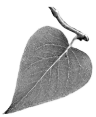
1. Calculate the area delimited by \(G_h\) and the angle bisector \(w\). Use this result to determine the area of the leaf, based on our model.

2. Determine the term of the tangent to \(G_h\) at the point \(\left(-2\left|h(-2)\right.\right)\). Calculate the angle between the two leaf edges at the leaf apex.

3. The current model does not describe well enough the shape of the upper leaf edge near the leaf apex. Therefore, we will use the graph \(G_k\) of a third order polynomial \(k\) in order to describe the upper leaf edge in the interval \(-2\leq x \leq 0\). The function \(k\) has to fulfill the following conditions (\(k'\) and \(h'\) are the derivatives of \(k\) and \(h\)):

   \[\begin{split}\mathrm{I} \qquad k(0)=h(0)\\ \mathrm{II} k'(0)=h'(0)\\ \mathrm{III} k(-2)=h(-2)\\ \mathrm{IV} k'(-2)=h'(-2)\\\end{split}\]

   Explain, why the conditions I, II and III are reasonable. Make plausible that the condition IV leads to a better description of the leaf edge near the leaf apex as compared to the first model.

Solution of part 3a

First, we want to calculate the area of the red region from part 2a. This can be done by subtracting the integrals of the functions \(h(x)\) and \(w(x)\) in the interval \(]-2;4[\):

\[\begin{split}\int\limits_{-2}^4 \left( h(x)-w(x) \right)\, \mathrm{d}x &= \int\limits_{-2}^4 \left( -\frac{1}{2}x^2+2x+4 -x \right)\mathrm{d}x\\ &= \int\limits_{-2}^4 \left( -\frac{1}{2}x^2+x+4 \right)\mathrm{d}x\\ &= \left[-\frac{1}{6}x^3+\frac{1}{2}x^2+4x\right]_{-2}^4\\ &=18\end{split}\]

This result can be verified with Sage:

Having obtained the heart-shaped figure by reflection of the red region at the angle bisector \(w\), the area enclosed by the heart-shaped figure is twice the red area. In view of the specified length scale, we obtain:

\[A_{\mathrm{Leaf}}=36\mathrm{cm}^2\]

Solution of part 3b

In order to determine the term of the tangent at the point \(\left(-2\left|h(-2)\right)\right.=(-2|-2)\), we first have to calculate the slope of the function \(h\) at the point -2. Using

\[h'(x) = -x+2\]

we obtain

\[m = h'(-2) = 4.\]

Inserting the point \(x=-2, y=-2\), the equation of the tangent \(y=m\cdot x+t\) becomes

\[y = 4x+6.\]

Using Sage, we can obtain this equation directly from the conditions that the tangent has to include the specified point and that the slope of the tangent has to equal the slope of the function \(h(x)\) at this point.

Further, we use Sage to draw the tangent into our figure.

The figure already indicates that the angle, based on our model, is considerably larger than the angle on the picture of the leaf. We can calculate the angle between the angle bisector and the tangent, based on their slopes \(m_w=1\) and \(m_t=4\) using the formula

\[\alpha = \arctan\left(\frac{m_t-m_w}{1+m_w m_t}\right) =\arctan\left(\frac{4-1}{1+4}\right) \approx 30,9°\]

The angle between the two edges is twice as large, i.e. approximately \(62°\).

Solution of part 3c

The conditions I and III are necessary for a continuous insertion of \(G_k\). Condition II ensures that the transition from \(h\) to \(k\) is smooth. Condition IV leads to a smaller angle between the leaf edges at the point (-2|-2) and therefore to a sharper leaf apex.

The problem did not ask for the exact solution of \(k\), but Sage will work this out for us:

We can use these parameters to plot the leaf according to the new model. The red curve is the new function \(k\).

Obviously, the new model fits the shape of the leaf better than the old model.