Linear Programming

The content of this book as well as quick search in the internet suggest that linear algebra is a branch of mathematics that concerns linear equations, linear operators and their matrix representations. Nevertheless it can be successfully applied to optimize a given expression under certain (linear) constraints. We illustrate some of the techniques, known as linear programming, on the following problems:

The diet problem

There are \(\ m\ \) different types of food, \(\ F_1,\ldots , F_m\ \), that supply varying quantities of the \(\ n\ \) nutrients, \(\ N_1,\ldots , N_n\ \), that are essential to good health. Let \(\ b_j\ \) be the minimum daily requirement of nutrient \(\ N_j\ \). Let \(\ c_i\ \) be the price of unit of food \(\ F_i\ \). Let \(\ a_{ji}\ \) be the amount of nutrient \(\ N_j\ \) contained in one unit of food \(\ F_i\ \). The problem is to supply the required nutrients at minimum cost.

In order to solve this problem we have to find the amount \(\ x_i\ \) of food \(\ F_i\ \), \(\ i\in\left\{ 1, 2,\ldots ,m\right\}\), that one have to buy so that the overall cost

\[c_1x_1 + \ldots + c_mx_m\]

is minimal and daily requirement for the nutrient \(\ N_j\) is satisfied:

\[a_{j1}x_1+ \ldots + a_{jm}x_m \geq b_j\,.\]

In other words, we have to solve the Standard Minimum Problem :

\[\begin{split}\begin{array} \text{minimize:} & c_1x_1 + \ldots + c_mx_m\\ \text{constraints:} & a_{j1}x_1+ \ldots + a_{jm}x_m \geq b_j\, ,\quad j\in\left\{ 1,\ldots ,n\right\}\\ & x_i\geq 0 \, ,\quad i\in\left\{ 1,\ldots ,m\right\}\\ \end{array}\end{split}\]

The last constraint represents the fact that one cannot buy a negative amount of food.

The optimal allocation problem

A company produces \(\ m\ \) types of products, \(\ P_1,\ldots , P_m\ \), out of \(\ n\ \) types of resources, \(\ R_1,\ldots , R_n\ \). One unit of the product \(\ P_i\ \) brings \(\ p_i\ \) of profit and requires \(\ a_{ji}\ \) units of the resource \(\ R_j\ \), \(\ i\in\left\{ 1, 2,\ldots ,m\right\}\, ,\ j\in\left\{ 1, 2,\ldots ,n\right\}\ \). The problem is to maximize the profit if there are only \(\ r_j\ \) units of the resource \(\ R_j\ \), \(\ j\in\left\{1,\ldots , n\right\}\ \).

This problem is very similar to the diet problem, but this time asks for optimal numbers \(\ x_i\ \) of products \(\ P_i\ \) that should be produced so that the profit is maximal. This represents the Standard Maximum Problem :

\[\begin{split}\begin{array} \text{maximize:} & p_1x_1 + \ldots + p_mx_m\\ \text{constraints:} & a_{j1}x_1+ \ldots + a_{jm}x_m \leq r_j\, ,\quad j\in\left\{ 1,\ldots ,n\right\}\\ & x_i\geq 0 \, ,\quad i\in\left\{ 1,\ldots ,m\right\}\\ \end{array}\end{split}\]

Note

Observe that to maximize the values of some function \(f(x)\) is the same as to minimize the values of \(-f(x)\). Therefore every standard maximum problem can be easily transformed to a standard minimum problem and vice versa:

\[\begin{split}\begin{array} \text{maximize:} & c_1x_1 + \ldots + c_mx_m \\ \text{constraints:} & a_{j1}x_1+ \ldots + a_{jm}x_m \leq b_j\, ,\quad j\in\left\{ 1,\ldots ,n\right\}\\ & x_i\geq 0 \, ,\quad i\in\left\{ 1,\ldots ,m\right\}\\ \end{array}\end{split}\]

is equivalent to

\[\begin{split}\begin{array} \text{minimize:} & -(c_1x_1 + \ldots + c_mx_m)\\ \text{constraints:} & -a_{j1}x_1- \ldots - a_{jm}x_m \geq -b_j\, ,\quad j\in\left\{ 1,\ldots ,n\right\}\\ & x_i\geq 0 \, ,\quad i\in\left\{ 1,\ldots ,m\right\}\\ \end{array}\end{split}\]

The Geometric Method

If the expression to minimize/maximize contains only 2 or 3 unknowns, the problem can be solved graphically.

Example 1.

One company produces two products \(P_1\) and \(P_2\) out of three resources \(R_1, R_2, R_3\). The amount of resources which are necessary for production as well as their availability is given in the following table:

	\(P_1\)	\(P_2\)	Availability
\(R_1\)	3	1	18
\(R_2\)	2	4	40
\(R_3\)	3	2	24

The profit from products \(P_1\) and \(P_2\) is respectively $2 and $3.

How many items of \(P_1\) and \(P_2\) should be produced so that the profit is maximal?

Denote by \(x\) and \(y\) the number of items of \(P_1\) and \(P_2\) respectively. The problem can be written in a concise form as

\[\begin{split}\begin{array} \text{maximize:} & 2x + 3y\\ \text{constraints:} & 3x+y \leq 18 \,,\\ & 2x+ 4y \leq 40 \,,\\ & 3x+ 2y \leq 24 \,,\\ & x, y\geq 0 \,.\\ \end{array}\end{split}\]

The constraints determine the feasible set of solutions to the problem. To draw this region, we first draw the lines which mark its boundaries, that is, \(\ y = 18-3x,\ 4y = 40-2x,\ 2y=24-3x\ \), and then mark the region below the lines (with \(x, y\geq 0\)):

sage: l1=plot(18-3*x, (x, 0, 7), fillcolor=(3/5, 4/5, 1),fill=0,legend_label='$18-3x$')
sage: l2=plot((40-2*x)/4, (x, 0, 7), color="purple", fillcolor=(4/5, 3/5, 1), fill='axis',legend_label='$(40-2x)/4$')
sage: l3=plot((24-3*x)/2, (x, 0, 7), color="green", fillcolor=(0,4/5,0), fill='axis',legend_label='$(24-3x)/2$')
sage: (l1+l2+l3).show(figsize=5, ymin=0)

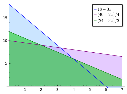
The picture tells us that the points \((x, y)\) that satisfy all the requirements lie in the polygon determined by the points \((0,0),(0,10),(2,9),(4,6),(6,0)\). We want to maximize the profit function \(\ p=2x+3y\ \). In order to find out for which values of \(x, y\) the constant \(p\) is biggest, we add a few lines \(\ 3y=p-2x\ \) to the picture above:

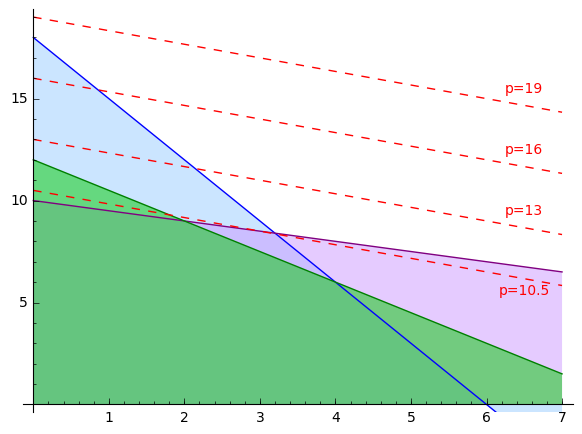
Now it’s clear that the maximal profit is obtained at the point \((x,y)=(2,9)\) as this is the point within the polygon which the line \(\ 3y=p-2x\ \) touches first. The point \((x,y)=(2,9)\) represents 2 items of the product \(P_1\) and 9 items of the product \(P_2\); the profit is \(\ p=2\cdot 2+3\cdot 9=$31\).

Example 2.

Consider the following diet problem:

Food	Cost/serving	Vitamin A (min 0.9 mg)	Iron (min 8 mg)	Calcium (min 1000 mg)
Corn	$ 0.18	0.009 mg	0.52 mg	2 mg
2% milk	$ 0.23	0.028 mg	0.02 mg	120 mg
Wheat bread	$ 0.05	0 mg	0.8 mg	20 mg

Denote by \(x, y\) and \(z\) the number of servings of corn, milk and bread, respectively. The problem of minimizing the expenditure while providing sufficient amount of vitamine A, iron and calcium may be summarized as follows:

\[\begin{split}\begin{array} \text{minimize:} & 0.18x + 0.23y + 0.05z\\ \text{constraints:} & 0.009x+0.028y \geq 0.9 \,,\\ & 0.52x+ 0.02y + 0.8z \geq 8 \,,\\ & 2x+ 120y + 20z\geq 1000 \,,\\ & x, y, z\geq 0 \,.\\ \end{array}\end{split}\]

Even though this problem can be still represented geometrically, it is much harder to see what the feasible set is and at which point the cost function \(\ c=0.18x + 0.23y + 0.05z\ \) achieves the minimum.

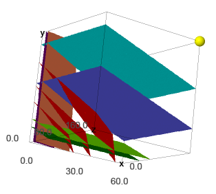
(To draw the picture we used the function implicit_plot3d().)

In this picture the cost surfaces are denoted by the red color. The first plane \(0.009x+0.028y= 0.9\) is marked by blue, the second by purple, and the last one by green color. The remaining three planes in lighter colours are parallel to the corresponding planes in darker colours and are drawn to facilitate picturing the feasible set; they show direction of the constraints. The yellow ball is the point with maximal coordinates at this picture: \((60,60,160)\).

The picture suggests that the place at which the red plane touches the feasible set first is located on the intersection of the blue and purple plane: the red planes that are closer to the origin do not contain any feasible points yet as they are below the restriction given by the blue plane.

We can compute the intersection of the planes using the formulae introduced in section Geometry of Linear Equations:

sage: var('x y z')
sage: eq1 = 0.009*x + 0.028*y == 0.9
sage: eq2 = 0.52*x + 0.02*y + 0.8*z == 8
sage: s = solve([eq1,eq2],[x,y,z])
sage: s

[[x == -1120/719*r1 + 10300/719, y == 360/719*r1 + 19800/719, z == r1]]

The solution is a line depending on parameter r1. We have to choose r1 so that the cost is minimal. First we substitute the solution to the inequality describing the third constraint to verify that it still holds; we obtain

\[\begin{split}\begin{align*} 2& \left(-\frac{1120}{719} r_1 + \frac{10300}{719}\right) +120\left( \frac{360}{719} r_1 + \frac{19800}{719}\right) +20r_1 -1000 \\ &= \frac{55340}{719} r_1 + \frac{1677600}{719} \end{align*}\end{split}\]

which is non-negative for every \(r_1\geq 0\) as required. At the same time, the cost turns out to be equal to

\[-0.115229485396384\, r_1 + 8.91237830319889\, .\]

It decreases with the growth of parameter \(r_1\). However, we can only increase \(r_1\) as long as \(x\) remains non-negative. The greatest possible \(r_1\) is when \(x=0\). The quickest way to find it is to use the function find_root() whose last two arguments denote the range of a variable:

We take \(z=r\) and under this assuption compute the intersection of the two planes, including also an equation for the cost function:

Since the cost remained positive after taking \(z=r\), it seems that the above solution solves our diet problem. However, since this time the picture was not as clear as in the previous example, this solution should be verified by using another method.

The last example already indicated demand for a more rigorous method. And of course, if the problem is more complex and deals with several variables (what often happens in practice), there is no way to obtain a good illustration of the problem. This is where linear algebra comes into play.

The Simplex Method

The algorithm was invented by an American mathematician George Dantzig in 1940s.

We demonstrate a solution of the Standard Minimum Problem with \(m\) unknowns \(x_1,\ldots, x_m\geq 0\) and \(n+m\) constraints:

\[\begin{split}\begin{array} \text{minimize:} & c_1x_1 + \ldots + c_mx_m\\ \text{constraints:} & a_{j1}x_1+ \ldots + a_{jm}x_m \geq b_j\, ,\quad j\in\left\{ 1,\ldots ,n\right\}\\ & x_i\geq 0 \, ,\quad i\in\left\{ 1,\ldots ,m\right\}\\ \end{array}\end{split}\]

which may be written in a matrix form as

\[\begin{split}\begin{array} \text{minimize:} & \boldsymbol{c}^T\boldsymbol{x}\\ \text{constraints:} & \boldsymbol{A}\boldsymbol{x} \geq \boldsymbol{b}\\ & \boldsymbol{x}\geq 0,\\ \end{array}\end{split}\]

where

\[\begin{split}\boldsymbol{c}\,=\,\left[\begin{array}{c} c_{1} \\ \vdots \\ c_{m} \end{array}\right]\,, \qquad \boldsymbol{x}\,=\,\left[\begin{array}{c} x_{1} \\ \vdots \\ x_{m} \end{array}\right]\,, \qquad \boldsymbol{A}\ =\ \left[\;\begin{array}{ccc} a_{11} & \ldots & a_{1m} \\ \vdots & \ddots & \vdots \\ a_{n1} & \ldots & a_{nm} \end{array}\right]\,, \qquad \boldsymbol{b}\,=\,\left[\begin{array}{c} b_{1} \\ \vdots \\ b_{n} \end{array}\right]\,,\end{split}\]

and by \(\ \boldsymbol{x}\geq 0\ \) (or \(\boldsymbol{A}\boldsymbol{x} \geq \boldsymbol{b}\)) we mean that each coordinate of the vector \(\ \boldsymbol{x}\ \) (or \(\boldsymbol{A}\boldsymbol{x}-\boldsymbol{b}\)) is greater or equal zero.

We will explain the consecutive steps along the way by referring to Example 1. discussed above, which we rewrite as the minimization problem:

\[\begin{split}\begin{array} \text{minimize:} & -2x -3y\\ \text{constraints:} & -2x -4y \geq -40 \,,\\ & -3x -2y \geq -24 \,,\\ & -3x-y \geq -18 \,,\\ & x, y\geq 0 \,.\\ \end{array}\end{split}\]

Step I:

Change the constraints \(\boldsymbol{A}\boldsymbol{x} \geq \boldsymbol{b}\) into equalities by introducing new variables.

Observe that the constraint \(\ \boldsymbol{A}\boldsymbol{x} \geq \boldsymbol{b}\ \) may be equivalently written as \(\ \boldsymbol{w} =\boldsymbol{A}\boldsymbol{x} - \boldsymbol{b}\, ,\quad \boldsymbol{w}\geq 0\ \). Therefore the following problems are equivalent:

\[\begin{split}\begin{cases} min\quad \boldsymbol{c}^T\boldsymbol{x}\\ \boldsymbol{A}\boldsymbol{x} \geq \boldsymbol{b}\\ \boldsymbol{x}\geq 0\end{cases} \qquad\Longleftrightarrow\qquad \begin{cases} min\quad \left[\begin{array}{c} \boldsymbol{c}^T & \boldsymbol{0}^T\end{array}\right] \left[\begin{array}{c}\boldsymbol{x}\\ \boldsymbol{w}\end{array}\right]\\ \left[\boldsymbol{A}\;\; -I\right]\left[\begin{array}{c}\boldsymbol{x}\\ \boldsymbol{w}\end{array}\right] =\boldsymbol{b}\\ \boldsymbol{x},\, \boldsymbol{w}\geq 0 \end{cases}\end{split}\]

We simplify our notation:

\(\left[\boldsymbol{A}\;\; -I\right]\) is renamed \(\ \boldsymbol{A}\ \), \(\ \ \left[\begin{array}{c}\boldsymbol{x}\\ \boldsymbol{w}\end{array}\right]\) is renamed \(\ \boldsymbol{x}\ \), \(\ \ \left[\begin{array}{c} \boldsymbol{c}\\ \boldsymbol{0}\end{array}\right]\) is renamed \(\ \boldsymbol{c}\ \),

so that we have to solve the problem

\[\begin{split}\begin{array} \text{minimize:} & \boldsymbol{c}^T\boldsymbol{x}\\ \text{constraints:} & \boldsymbol{A}\boldsymbol{x} = \boldsymbol{b}\\ & \boldsymbol{x}\geq 0,\\ \end{array}\end{split}\]

where \(\boldsymbol{A}\) is \(n\times (m+n)\) matrix and \(x\) has \(m+n\) components. We will call \(\boldsymbol{c}^T\boldsymbol{x}\) the cost function.

Example.

In case of Example 1., we obtain

\[\begin{split}\boldsymbol{A}=\left[\begin{array}{ccccc} -2 & -4 & -1 & 0 & 0\\ -3 & -2 & 0 & -1 & 0\\ -3 & -1 & 0 & 0 & -1\\ \end{array}\right],\qquad \boldsymbol{b}=\left[\begin{array}{c} -40 \\ -24 \\ -18 \end{array}\right],\qquad \boldsymbol{c}=\left[\begin{array}{c} -2 \\ -3 \\ 0 \\ 0 \\ 0 \end{array}\right],\qquad \boldsymbol{x}=\left[\begin{array}{c} x \\ y \\ w_1 \\ w_2 \\ w_3 \end{array}\right].\end{split}\]

Step II:

Find a point that satisfies the constraints.

It is convenient to write down the data in the tableau: \(\ T=\left[\begin{array}{cc} \boldsymbol{A} & \boldsymbol{b}\\ \boldsymbol{c} & 0\end{array}\right]\). Recall that \(\boldsymbol{A}\) is \(n\times (m+n)\) matrix, and so it may be written as \([\boldsymbol{B}\;\; \boldsymbol{N}]\ \) where \(\boldsymbol{B}\) is a square matrix of size \(n\), and \(\boldsymbol{N}\) is \(n\times m\) matrix. Similarly, we can write \(\ \boldsymbol{c}=\left[\begin{array}{c}\boldsymbol{c_B}\\ \boldsymbol{c_N}\end{array}\right]\), \(\ \boldsymbol{x}=\left[\begin{array}{c}\boldsymbol{x_B}\\ \boldsymbol{x_N}\end{array}\right]\), where \(\boldsymbol{c_B}\), \(\boldsymbol{x_B}\) and \(\boldsymbol{c_N}\), \(\boldsymbol{x_N}\) have respectively \(n\) and \(m\) components. In this way,

\[\begin{split}T=\left[\begin{array}{cccc} \boldsymbol{B} & \boldsymbol{N} & | & \boldsymbol{b}\\ \boldsymbol{c_B}^T & \boldsymbol{c_N}^T & | & 0\end{array}\right]\,,\qquad \boldsymbol{x}=\left[\begin{array}{c} \boldsymbol{x_B} \\ \boldsymbol{x_N}\end{array}\right],\end{split}\]

which should be interpreted as

\[\begin{split}\left[\begin{array}{cc} \boldsymbol{B} & \boldsymbol{N}\end{array}\right] \left[\begin{array}{c} \boldsymbol{x_B} \\ \boldsymbol{x_N}\end{array}\right] =\boldsymbol{b}\,,\qquad\text{minimize:}\;\; \left[\begin{array}{cc} \boldsymbol{c_B}^T & \boldsymbol{c_N}^T\end{array}\right] \left[\begin{array}{c} \boldsymbol{x_B} \\ \boldsymbol{x_N}\end{array}\right]\, .\end{split}\]

In order to find a point \(\boldsymbol{x_B}\) which satisfies the constraints of the problem it suffices to perform Gauss Jordan elimination on the first \(n\) rows of \(T\) (i.e., excluding the last row) so that the submatrix \([\boldsymbol{B}\; \boldsymbol{N}]\) is in reduced row echelon form. This is equivalent to multiplication of these rows by \(\boldsymbol{B}^{-1}\) on the left. We obtain:

\[\begin{split}T=\left[\begin{array}{cccc} \boldsymbol{I} & \boldsymbol{B}^{-1}\boldsymbol{N} & | & \boldsymbol{B}^{-1}\boldsymbol{b}\\ \boldsymbol{c_B}^T & \boldsymbol{c_N}^T & | & 0\end{array}\right]\,,\end{split}\]

which means that

\[\boldsymbol{x_B} = -\boldsymbol{B}^{-1}\boldsymbol{N}\boldsymbol{x_N}+\boldsymbol{B}^{-1}\boldsymbol{b}\,.\]

Hence, the problem to minimize the quantity \(\ \boldsymbol{c_B}^T\boldsymbol{x_B}+\boldsymbol{c_N}^T\boldsymbol{x_N}\ \) becomes

\[\text{minimize:}\qquad (-\boldsymbol{c_B}^T\boldsymbol{B}^{-1}\boldsymbol{N}+\boldsymbol{c_N}^T)\boldsymbol{x_N} +\boldsymbol{c_B}^T\boldsymbol{B}^{-1}\boldsymbol{b}\, .\]

Example.

In Example 1.,

\[\begin{split}T=\left[\begin{array}{ccccccc} -2 & -4 & -1 & 0 & 0 & | & -40\\ -3 & -2 & 0 & -1 & 0 & | & -24\\ -3 & -1 & 0 & 0 & -1 & | & -18\\ -2 & -3 & 0 & 0 & 0 & | & 0\\ \end{array}\right]\,.\end{split}\]

We use Sage to determine \(\boldsymbol{x_B}\) and current cost.

sage: B=Matrix([[-2,-4,-1],[-3,-2,0],[-3,-1,0]])
sage: N=Matrix([[0,0],[-1,0],[0,-1]])
sage: b=Matrix([[-40],[-24],[-18]])
sage: cB=Matrix([-2,-3,0])
sage: cN=Matrix([0, 0])
sage: T=block_matrix(QQ,[[B,N,b],[cB, cN, 0]])
sage: T

[ -2  -4  -1|  0   0|-40]
[ -3  -2   0| -1   0|-24]
[ -3  -1   0|  0  -1|-18]
[-----------+-------+---]
[ -2  -3   0|  0   0|  0]

Before we proceed, let’s look what is actually happenning. The above table means that we are looking for a solution of the following system of equations:

\[\begin{split}\begin{alignat*}{7} -2x & \, - \, 4y & \, - \, w_1 & & & \; =\; & -40 \\ -3x & \, - \, 2y & & \, - \, w_2 & & \; =\; & -24 \\ -3x & \, - \, y & & & \, - \, w_3 & \; =\; & -18 \end{alignat*}\end{split}\]

This can be rewritten in a column picture, so that we obtain an equality between a vector and a linear combination of five three-dimensional vectors:

\[\begin{split}\left[\begin{array}{r} -2\\ -3\\ -3\end{array}\right] x + \left[\begin{array}{r} -4\\ -2\\ -1\end{array}\right] y + \left[\begin{array}{r} -1\\ 0\\ 0\end{array}\right] w_1 + \left[\begin{array}{r} 0\\ -1\\ 0\end{array}\right] w_2 + \left[\begin{array}{r} 0\\ 0\\ -1\end{array}\right] w_3 = \left[\begin{array}{r} -40\\ -24\\ -18\end{array}\right]\end{split}\]

However, two of the vectors on the left may be expressed in terms of the three other vectors (see Theorem 5 in Dimension of a Vector Space or Fundamental Concepts in Linear Algebra for a proof of Theorem 5). Hence the division in the table: at the first stage \(\ w_2,\, w_3\ \) serve as parameters and will guide us later how to optimize the cost function.

If we set \(w_2=w_3=0\), the above equation means that we restrict our attention to the plane spanned by the first three vectors (or in other words: generated by the points \(\ (-2,-3,-3),\, (-4,-2,-1),\, (-1,0,0)\ \)) and look for constants \(x,y,w_1\) so that the linear combination

\[\begin{split}\left[\begin{array}{r} -2\\ -3\\ -3\end{array}\right] x + \left[\begin{array}{r} -4\\ -2\\ -1\end{array}\right] y + \left[\begin{array}{r} -1\\ 0\\ 0\end{array}\right] w_1\end{split}\]

is equal to \(\boldsymbol{b}=\left[\begin{array}{ccc} -40 & -24 & -18\end{array}\right]^T\).

From another point of view, coming back to the row picture (but with \(w_2=w_3=0\)), the system of equations

\[\begin{split}\begin{alignat*}{5} -2x & \, - \, 4y & \, - \, w_1 & \; =\; & -40 \\ -3x & \, - \, 2y & & \; =\; & -24 \\ -3x & \, - \, y & & \; =\; & -18 \end{alignat*}\end{split}\]

may be interpreted by picture from Example 1: it represents the intersection point of the blue and the green line under the additional condition that this point is under the purple line.

In order to find \(x,y,w_1\), we multiply the matrix \(T\) by \(\ \left[\begin{array}{cc} \boldsymbol{B}^{-1} & \boldsymbol{0}\\ \boldsymbol{0} & 1 \end{array}\right]\ \):

sage: T=block_matrix([[B.inverse(),zero_matrix(3,1)],[zero_matrix(1,3),1]])*T
sage: T

[    1     0     0| -1/3   2/3|    4]
[    0     1     0|    1    -1|    6]
[    0     0     1|-10/3   8/3|    8]
[-----------------+-----------+-----]
[   -2    -3     0|    0     0|    0]

Hence,

\[\begin{split}\begin{alignat*}{3} x &\; =\; & \frac13 w_2 &\, -\,\frac23 w_3 & \, +\, 4\\ y &\; =\; & -w_2 & \, +\, w_3 &\, +\, 6\\ w_1 &\; =\; & \frac{10}{3} w_2 & \, -\,\frac83 w_3 & \, +\, 8 \end{alignat*}\end{split}\]

and if we set \(w_2=w_3=0\), we obtain \((x,y,w_1)=(4,6,8)\) which corresponds to the point \((4,6)\), the intersection of the blue and the green line, as expected.

The cost at this corner is equal to

\[\begin{split}\left[\begin{array}{ccc} -2 & -3 & 0 \end{array}\right] \left[\begin{array}{c} 4 \\ 6\\ 8 \end{array}\right] = -26 .\end{split}\]

However, if we do not specialise to \(w_2=w_3=0\) but rather allow these parameters to vary, we obtain the actual cost:

\[\begin{split}\left[\begin{array}{ccc} -2 & -3 & 0 \end{array}\right] \left[\begin{array}{c} x \\ y\\ w_1 \end{array}\right] = -2\left(\frac13 w_2 -\frac23 w_3\right)-3\left(-w_2 + w_3\right)+0\left(\frac{10}{3} w_2 -\frac83 w_3\right) =\frac73 w_2 -\frac53 w_3 -26\, .\end{split}\]

Since we require \(w_2, w_3\geq 0\), it is clear that taking \(w_3> 0\) will reduce the cost. Geometrically, this means that the point \((x,y)\) should be allowed to be strictly under the blue line.

Step III:

Is the cost at this point lowest possible?

In Step II we obtained the point \(\boldsymbol{x_B} = -\boldsymbol{B}^{-1}\boldsymbol{N}\boldsymbol{x_N}+\boldsymbol{B}^{-1}\boldsymbol{b}\) which satisfies the contraints of the problem. However, the corresponding cost

\[(\boldsymbol{c_N}^T-\boldsymbol{c_B}^T\boldsymbol{B}^{-1}\boldsymbol{N})\boldsymbol{x_N} +\boldsymbol{c_B}^T\boldsymbol{B}^{-1}\boldsymbol{b}\]

may not be minimal. As long as one of the entries of \(\ \boldsymbol{c_N}^T-\boldsymbol{c_B}^T\boldsymbol{B}^{-1}\boldsymbol{N}\ \) is negative, it is possible to choose the corresponding entry of \(\ \boldsymbol{x_N}\ \) to be non-zero and thus reduce the cost. If \(\ \boldsymbol{c_N}^T-\boldsymbol{c_B}^T\boldsymbol{B}^{-1}\boldsymbol{N}\geq 0\ \), then the cost at the point \(\boldsymbol{x}\) is minimal and is equal to \(\ \boldsymbol{c}^T\boldsymbol{x}\ \).

The above considerations justify the next operation on rows of the tableau \(T\):

subtract from the last row the product of \(\boldsymbol{c_B}\) and the first \(n\) rows,

\[\begin{split}\left[\begin{array}{cc} \boldsymbol{I} & \boldsymbol{0}\\ -\boldsymbol{c_B}^T & 1\end{array}\right]\cdot \left[\begin{array}{cccc} \boldsymbol{I} & \boldsymbol{B}^{-1}\boldsymbol{N} & | & \boldsymbol{B}^{-1}\boldsymbol{b}\\ \boldsymbol{c_B}^T & \boldsymbol{c_N}^T & | & 0\end{array}\right] =\left[\begin{array}{cccc} \boldsymbol{I} & \boldsymbol{B}^{-1}\boldsymbol{N} & | & \boldsymbol{B}^{-1}\boldsymbol{b}\\ \boldsymbol{0} & \boldsymbol{c_N}^T-\boldsymbol{c_B}^T\boldsymbol{B}^{-1}\boldsymbol{N} & | & -\boldsymbol{c_B}^T\boldsymbol{B}^{-1}\boldsymbol{b}\end{array}\right]\,.\end{split}\]

Example

We apply the above operation to the matrix \(T\) from our example:

sage: T=block_matrix(QQ,[[identity_matrix(3),zero_matrix(3,1)],[-cB,1]])*T
sage: T

[    1     0     0| -1/3   2/3|    4]
[    0     1     0|    1    -1|    6]
[    0     0     1|-10/3   8/3|    8]
[-----------------+-----------+-----]
[    0     0     0|  7/3  -5/3|   26]

Since the submatrix corresponding to \(\ \boldsymbol{c_N}^T-\boldsymbol{c_B}^T\boldsymbol{B}^{-1}\boldsymbol{N}\ \) contains a negative number:

sage: T.subdivision(1,1)

[ 7/3 -5/3]

the current cost \(-26\) is not minimal.

Step IV:

If the cost is not minimal, change the basis.

Assume that the \(i\)-th entry of \(\ \boldsymbol{c_N}^T-\boldsymbol{c_B}^T\boldsymbol{B}^{-1}\boldsymbol{N}\ \) is negative. Hence, in order to reduce the cost we should include \(x_{N,i}\) to the basis. This means that we have to exclude another variable. Which variable should be excluded so that the cost is reduced?

Compare the quotients of the entries of the last column \(\boldsymbol{B}^{-1}\boldsymbol{b}=\left[b_1', b_2',\ldots, b_n'\right]^T\) and the \(i\)-th column of \(\boldsymbol{B}^{-1}\boldsymbol{N}=[r_{v\nu}]\ \): \(\ \begin{array}{cccc} \frac{b_1'}{r_{1i}}, & \frac{b_2'}{r_{2i}}, &\ldots, & \frac{b_n'}{r_{ni}}\end{array}\ \). For simplicity assume that the smallest positive is the \(1\)-st quotient \(\frac{b_1'}{r_{1i}}\). In this case we exchange the \(1\)-st column of the tableau \(T\) with the \(n+i\)-th column, so that:

\[\begin{split}T=\left[\begin{array}{ccccccccccc} r_{1i} & 0 & \ldots & 0 & r_{11} & \ldots & 1 & \ldots & r_{1m} & | & b_1'\\ r_{2i} & 1 & \ldots & 0 & r_{21} & \ldots & 0 & \ldots & r_{2m} & | & b_2'\\ \vdots & \vdots & \ddots & \vdots & \vdots & \ddots & \vdots & \ddots & \vdots & | & \vdots\\ r_{ni} & 0 & \ldots & 1 & r_{n1} & \ldots & 0 & \ldots & r_{nm} & | & b_n'\\ c_i' & 0 & \ldots & 0 & c_1' & \ldots & 0 & \ldots & c_m' & | & -\boldsymbol{c_B}^T\boldsymbol{B}^{-1}\boldsymbol{b} \end{array}\right]\end{split}\]

where \(\ \boldsymbol{c_N}^T-\boldsymbol{c_B}^T\boldsymbol{B}^{-1}\boldsymbol{N} = \left[c_1', c_2',\ldots, c_m'\right]\).

Note that one of the things that we have to do in order to write \(T\) in reduced row echelon form is to divide each row of the matrix by the entries from the first column; this will make the last column equal to \(\left[\frac{b_1'}{r_{1i}}, \frac{b_2'}{r_{2i}},\ldots, \frac{b_n'}{r_{ni}}\right]^T\) and because now only the first entry of first \(n\) entries in the last row of \(T\) is non-zero, only \(\frac{b_1'}{r_{1i}}\) will contribute to the cost.

Example

As we noticed above, allowing \(w_3>0\) (or, in other words, allowing the point \((x,y)\) to be strictly under the blue line) wil reduce the cost. Moreover, the plane corresponding to the cost function \(\boldsymbol{c}^T\boldsymbol{x}\) will touch the feasible set first on the boundary (and in most cases, the corner of the set). Last time we reached the point \((4,6)\). Decision to stay under the blue line should correspond to moving up along the green line to the point \((2,9)\).

First we compute the quotients of the entries in the last column and the column above \(-\frac53\) of the matrix \(T\).

sage: for i in range(3):
sage:     print T[i][5]/T[i][4]

6
-6
3

The smallest positive is the third quotient. Observe that the third column of \(T\) corresponds exactly to the additional variable \(w_1\). Hence, if we exhange the third column of the matrix \(T\) with the fifth column, we do not lose variables \(x,y\); the only thing that changes is that now we allow to be under the blue line and want to stay on the border of the purple line.

sage: T.swap_columns(2,4)
sage: T

[    1     0   2/3| -1/3     0|    4]
[    0     1    -1|    1     0|    6]
[    0     0   8/3|-10/3     1|    8]
[-----------------+-----------+-----]
[    0     0  -5/3|  7/3     0|   26]

We perform the steps II and III again.

sage: T=block_matrix([[T.subdivision(0,0).inverse(),zero_matrix(3,1)],[zero_matrix(1,3),1]])*T

[   1    0    0| 1/2 -1/4|   2]
[   0    1    0|-1/4  3/8|   9]
[   0    0    1|-5/4  3/8|   3]
[--------------+---------+----]
[   0    0 -5/3| 7/3    0|  26]

sage: T=block_matrix(QQ,[[identity_matrix(3),zero_matrix(3,1)],[-T.subdivision(1,0),1]])*T
sage: T

[   1    0    0| 1/2 -1/4|   2]
[   0    1    0|-1/4  3/8|   9]
[   0    0    1|-5/4  3/8|   3]
[--------------+---------+----]
[   0    0    0| 1/4  5/8|  31]

As we can see, now all the entries of the last row are positive, and thus the cost cannot be reduced further. The minimal cost equals \(\ -31\ \) and is achieved at the point \(\ (2,9)\ \) as expected. Since we changed the original problem of maximization to minimization, the original cost we wanted to compute is \(\ -(-31)=31\ \).

Step V:

Repeat the steps II-IV until the cost is minimal.

The above explanation was partially inspired by an excellent lecture of prof. Craig Tovey, professor in the Georgia Tech Stewart School of Industrial and Systems Engineering. The reader is encouraged to watch that lecture for further clarification.

Exercises

Since the solutions of the exercises below require writing a lot of code, it may be better to download them from here in a form of a notebook and then open them e.g. via CoCalc available here

Exercise 1.

One school organizes a trip for 250 people. A shipping company offers coaches of types A, B, C which can take 32, 45 and 60 people resepctively, and cost 600, 800 and 1000 euros respectively. Find out how many coaches of each type the school should hire so that the cost is minimal.

Exercise 2.

Consider the diet problem from Example 2. Use simplex method to verify whether the solution obtained by the geometric method is correct.

Exercise 3.

A company Woolwear produces jackets, sweaters and shirts out of wool (\(60\) units), cotton (\(100\) units), zips (\(50\) units), buttons (\(60\) units) and fur (\(60\) units). The following table presents the number of units of each material that is necessary for a production of a given type of clothing:

	Wool	Cotton	Zip	Button	Fur
Sweater	2	5	1	0	1
Jacket	1	7	0	2	3
Shirt	1	1	3	3	1

Each sweater gives \(20\) euros of profit, jacket gives \(30\) euros of profit, and shirt \(10\). How many sweaters, jackets and shirts the company should produce out of available materials in order to obtain a maximal profit?

Note

The simplex method does not necesarily produce integer solutions; this may be the case for this problem. Try to round the solutions to integer values which satisfy the constraints and so that the resulting profit differs from the optimal one by less than \(10\) (note that the profit is always the number divisible by \(10\)).

In general, a linear programming problem where one seeks an integer solution is called an integer programming problem. See wikipedia page for a description and a list of possible algorithms. In fact, in contrast to linear programming problems which can be solved efficiently, integer programming problems are in may cases NP-hard.