Epidemic model of Kermack-McKendrick

Epidemic means a widespread outbreak of an infectious disease and many people are infected at the same time. The global epidemic is called pandemic, i.e. it exists in almost all of an area or in almost all of a group of people, animals, or plants.

Panˈdemik/:

pan means “all”; demic (or demographic) means “people.”

Throughout history, there have been a number of pandemics, such as smallpox and tuberculosis. One of the most devastating pandemics was the Black Death, which killed over 75 million people in 1350. The most recent pandemics include the HIV pandemic as well as the 1918 and 2009 H1N1 pandemics.

• In 1918, the virulent Spanish flu left 50 to 100 million people dead. Though mostly forgotten, it has been called “the greatest medical holocaust in history.”

• the Asian flu of 1958 and 1959 had a global death toll as high as 2 million and an estimated 70,000 of those in the US alone.

• Early in 1968, the Hong Kong flu began. By September, it made its way around the world, including the United States, and became widespread by December. It is believed that the number of those infected peaked during the fall, when kids were at school, transmitting the virus more freely. Still, as many as a million people died, 34,000 in the US alone between September 1968 and March 1969.

As usually we start modeling assuming simplified conditions. We consider an isolated population which is divided into three compartments:

1. Individuals who can catch the decease; their population is denoted by \(S\). These are called susceptible individuals or susceptibles

2. Infectives \(I\) who have the decease and can transmit it.

3. Individuals \(R\) who have recovered and cannot contract the disease again. In ths group there are ibdividuals who are immune or isolated until recovered. They are called removed/recovered individuals.

The total population size \(N\) is constant and is the sum of the sizes of these three groups:

\[S + I + R = N = const. \quad \quad \mbox{constant number of members in the population}\]

We want to derive differential equations which determine how three groups change over time. When a susceptible individual enters into contact with an infectious individual, that susceptible individual becomes infected with a certain probability and moves from the susceptible class into the infected class. The susceptible population \(S\) decreases in a unit of time by all individuals who become infected in that time. It means that

\(\frac{dS}{dt} = -b_0 S < 0\).

At the same time, the class of infectives increases by the same number of newly infected individuals and those individuals who recover or die leave the infected class:

\(\frac{dI}{dt} = c_0 I - a I\)

Individuals who recover leave the infectious class \(I\) and move to the recovered class \(R\) and its number grows:

\(\frac{dR}{dt} > 0\)

The modeling is based on the Malthus model: increases-decreases or birth-death. Moreover, as for the Lotka-Volterra system, we have to think about the rates \(b_0\) and \(c_0\). The rate \(b_0\) should depend on the number \(I\): if more infecious then the greater probability to become infecious for individuals from the group \(S\). So, we can assume that \(b_0 = bI\). The similar argumentation can be performed for the rate \(c_0 = c S\).

We have to construct evolution equations in the way to preserve the constant number of all individuals in the population \(N\). It leads to the set of equations:

\[\frac{dS}{dt} = - r I S , \quad \quad \frac{dI}{dt} = r S I -aI, \quad \quad \frac{dR}{dt} = aI\]

Therefore we have to take for the rates \(b = c \equiv r\) and in the third equation for \(R\) the term in the right hand side has to be \(+ aI\). Indeed, if we add equations then

\[\begin{split}\begin{aligned} \frac{dS}{dt} + \frac{dI}{dt} + \frac{dR}{dt} = \frac{d(S + I + R)}{dt} = 0 \quad \quad \Rightarrow \quad \quad S + I + R = const. \quad \quad \Rightarrow \\ S(t) + I(t) + R(t) = const. = S(0) + I(0) + R(0) = N_0 \end{aligned}\end{split}\]

As it is seen, the total number of individuals \(S(t) + I(t) + R(t)\) in the population is constant and determined by the initial conditions \(S(0) + I(0) + R(0)\). In this way, the above set of three equations are in accordance with the assumption on the isolated population. The model can be modified in various ways and everybody can form its own model. Another problem is whether it can describe a piece of any reality.

This model is called the Kermack-McKendrick model and it was proposed in 1927. This model can describe the epidemic phenomenon if \(S(t)\) will grow in some interval of time \([0, t_c]\). After time \(t_c\) epidemic can be stoped or not. If \(S(t)\) will be a decreasing function of time then it cannot describe epidemic. In this model, there two parameters: the infection rate \(r>0\) and the removal (recovery) rate \(a >0\) which have the unit \([1/second]\).

Two first equations form a closed set of differential equations:

\[\frac{dS}{dt} = - r S I, \quad S(0) = S_0 > 0 \quad \quad \frac{dI}{dt} = r S I -aI = I (r S - a), \quad I(0) =I_0 >0\]

If \(I(t)\) is found from this set of equations then the third equation has the solution

\[R(t) = a \int_0^t I(u) du, \quad R(0) =0\]

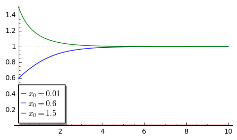
Now, we will apply the method of stationary states. Putting the time derivatives zero, from the above set of two differential eqations we get algebraic equations for the stationary states:

\[I = 0 \quad \quad \quad S = \frac{a}{r}\]

Let us now calculate the corresponding Jacobi matrix:

\[\begin{split}\begin{aligned} \quad \quad \quad \quad J (S, I) = \begin{bmatrix}-r I& -r S\\ r I & r S - a \end{bmatrix} \quad \quad \mbox{in the stationary state:} \quad J= J\left(\frac{a}{r}, 0\right) = \begin{bmatrix}0&-a\\ 0&0 \end{bmatrix} \end{aligned}\end{split}\]

We determine its eigenvalues from the equation \(|J-\lambda I|=0\). Simple calculation show that the eigenvalues are zero! It means that the linearization method fails and cannot be applied. We will use the direct method and use SAGE. There are two parameters: the infection rate \(r\) and the removal rate \(a\). They should decide about the tempo of epidemic. It appears that not only \(r\) and \(a\) decide but also initial conditions. Below we present two set of parameters and the same initial conditions.

Example of a set of parameters

Two parameters: \(r\) and \(a\) decide about the epidemicc. As a first example, we assume the relation:

\[r \lt a\]

The infection rate \(R\) is smaller than the removal rate \(r\)

var('S I R') ## in this part the set of differential equations is solved nmerlcally
r,a = 1,2
T = srange(0, 3,0.01)
sol=desolve_odeint( vector([-r*S*I,r*S*I - a*I, a*I]), [2,1,0.5],T,[S,I,R])
line( zip ( T,sol[:,0]) ,figsize=(8,4),legend_label="S (susceptible)") +\
 line( zip ( T,sol[:,1]) ,color='red',legend_label="I (infective)")+\
 line( zip ( T,sol[:,2]) ,color='green',legend_label="R (recovered)")

We change the relation between the parameters:

\[r \gt a\]

The infection rate \(r\) is greater than the removal (recovery) rate \(a\)

var('S I R')
r1,a1 = 4,0.5
T = srange(0,3,0.01)
sol=desolve_odeint( vector([-r1*S*I,r1*S*I - a1*I, a1*I]), [2,1,0.5],T,[S,I,R])
line( zip ( T,sol[:,0]) ,figsize=(8,4),legend_label="S (susceptible)") +\
 line( zip ( T,sol[:,1]) ,color='red',legend_label="I (infective)")+\
 line( zip ( T,sol[:,2]) ,color='green',legend_label="R (recovered)")

The above two sets of parameters lead to two different time evolution. Why? To solve this question, let us consider the equation:

\[\frac{dI}{dt} = r S I -aI = I (r S - a)\]

The initial time evolution depends on the signe of derivative with respect to time \(t \to 0\). We know that if the derivative is positive then the function increases; if it is negative then the function decreases.

The sign of derivative at zero time is :

\[\frac{dI}{dt}|_{t=0} = r S(0) I(0) - a I(0) = I(0) [r S(0) - a]\]

If \(r S(0) - a \gt 0\) then the function \(I(t) \gt I(0)\) increases and one can observe epidemic. If \(r S(0) - a \lt 0\) then the function decreases \(I(t) \lt I(0)\) and epidemic is not observed. IN this phenomen one can note existence of the the threshold value:

\[S_c = \frac{a}{r}\]

If at initial time \(S(0) \gt S_c\) ** then epidemic occurs!**

The occurence of epidemic depends on how large is the population susceptible to infection. The population should be sifficiently large \(S(0) > S_c\) and its minimal value \(S_c = a/r\) depends on the relation of the removal rate \(a\) and the infection rate \(r\). It is the most important conclusion of this part.

Example of epidemic

The above model was applied to description of the flu epidemic in 1978 roku in one of the bey’s school with total of 763 boys.

Here are data:

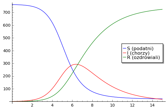
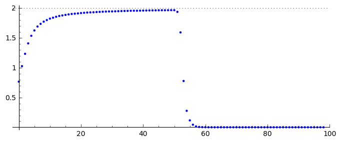
All boys: 763. One boy initiated the epidemic which lasted from 22 January to 4 February. In this time 512 boys were ill. In the sixth day it was the maximum of epidemic: 300 were ill. In the next days the number of infected started to decrease. From the date, it was possible to fit parameters of the model:

\[r = 0.00218, \quad \quad \quad S_c = 202.\]

Show all curves in the Kermack-McKendrick model for this set of parameters.

var('S I R')
r2,s = 0.00218, 202
T = srange(0,15,0.01)
sol=desolve_odeint( vector([-r2*S*I,r2*I*(S - s),r2*s*I]), [762,1,0],T,[S,I,R])
line( zip ( T,sol[:,0]) ,figsize=(6,4),legend_label="S (podatni)") +\
 line( zip ( T,sol[:,1]) ,color='red',legend_label="I (chorzy)")+\
 line( zip ( T,sol[:,2]) ,color='green',legend_label="R (ozdrowiali)")

Geographical spread of epidemic

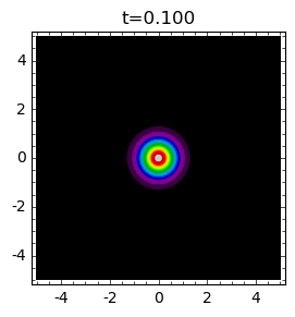
In the previous modeling we were interested in the time evolution of epidemic. The population was closed, not interacting with the “external” world as in the example of boys in the school. The spread of epidemic in territory has not been taken into account. Now, we want to present models of the epidemic with spread on given area. One of the models of spread in territory can be described as a process of diffusion. From mathematical point of view, the process of diffusion is determined by the Laplace operator. Usually, one can add the Laplace operators \(\Delta\) to the deterministic equations, here, to the Karmack-McKendrick equations:

\[\frac{\partial S }{\partial t} = -r S I + D_s \Delta S\]

\[\frac{\partial I }{\partial t} = r S I - a I + D \Delta I\]

where \(S = S(\vec r, t) = S(x, y, y)\) and \(I = I(\vec r, t)=I(x, y, t)\) describes concentrations of the population at time \(t\) in the point \(\vec r = (x, y)\) on the XY-plane. Parameters \(D_s\) and \(D\) are diffusion coefficients and describes tempo of population changes on the XY-plane for the population \(S\) and \(I\). We note that the diffusion process is determined by the Laplace operator \(\Delta\), i.e.

\[\Delta S(\vec r, t) = \left[\frac{\partial^2 }{\partial x^2} + \frac{\partial^2 }{\partial y^2} \right] S (\vec r, t) = \frac{\partial^2 S(x, y, t)}{\partial x^2} + \frac{\partial^2 S(x, y, t)}{\partial y^2}\]

In simpler models diffusion can be only in one dimension (in one direction). If we are not interest in the spatial spread of susceptible individuals \(S\) but only infectives \(I\) then it is sufficient to consider the model:

\[\frac{\partial S }{\partial t} = -r S I\]

\[\frac{\partial I }{\partial t} = r S I - a I + D \Delta I\]

This model was applied for modeling of spread of rabies among animals, in particuler among foxes. foxes. Model tego

The above model can be modified. For example, we can take into account the growth process of susceptible individuals \(S\), then, e.g.,

\[\frac{\partial S }{\partial t} = -r S I + B S \left(1-\frac{S}{S_0}\right)\]

\[\frac{\partial I }{\partial t} = r S I - a I + D \Delta I\]

In the first equation we recognize the Verhulst term describing the growth process of susceptible individuals \(S\). Parameters \(B\) and \(S_0\) have the same interpretation as in the Verhulst model: \(B\) characterizes the growth rate of population and \(S_0\) is the carrying capacity.

In this last model, there are 6 parameters. We sholud perfom the scaling to reduce their number. We define the following dimensionless variables and parameters:

\[U = \frac{S}{S_0}, \quad \quad V = \frac{r I}{B S_0}, \quad \quad y = \left(\frac{B}{D}\right)^{1/2} x , \quad \quad \tau = B t, \quad \quad \lambda = \frac{a}{r S_0}, \quad \quad \alpha = \frac{r S_0}{B}\]

In this rescaled variables the equations read:

\[\frac{\partial U }{\partial t} = U (1 - U - V)\]

\[\frac{\partial V }{\partial t} = \alpha V ( U - \lambda) + \Delta V\]

As we see only 2 parameters are relevant in this model. They occur only in the second equation.

Realistic modeling of spatial epidemic spread

Models can be extended taking into account the following factors:

1. Epidemic in homogeneous media

2. Epidemic in non-homogeneous media:

   • Obstacles as reflected walls distributed deterministically or randomly

   • Obstacles as sources or sinks. > There are two examples. In the first, sources can be implemented. In the second, complex geometry with the von Neumann boundary condition can be implemented.

var('u,v')
lam = .3
T = srange(0,45,0.01)
sol=desolve_odeint( vector([-a*u*v,a*v*u-lam*a*v]), [1,0.1],T,[u,v])
uvt = line( zip ( T,sol[:,0]) ,figsize=4,legend_label="S (podatni)") +\
 line( zip ( T,sol[:,1]) ,color='red',legend_label="I (chorzy)")
line( sol,figsize=4 )

Model of epidemic spread in homogeneous media

%timeit
import numpy as np
sparse = True
slicing = True
Dyf_u = .0
Dyf_v = 1.02
Dyf = max(Dyf_u,Dyf_v)
a = 1.0
lam = .3
l = 100.0 # dlugosc ukladu
t_end = 200 # czas symulacji
N = 160 # dyskretyzacja przestrzeni
h = l/(N-1)
dt = 0.052/(Dyf*(N-1)**2/l**2) # 0.2 z warunku CFL, krok nie moze byc wiekszy
dt_dyn = 0.02
print "dt,dt_dyn",dt,dt_dyn
dt = min(dt,dt_dyn)
sps = int(1/dt) # liczba krokow na jednostke czasu
Nsteps=sps*t_end  # calkowita liczba krotkow
print "sps=",sps,"dt=",dt,'Nsteps=',Nsteps
# warunek poczatkowy
u = np.zeros((N,N))
v = np.zeros((N,N))
u[:,:]=1.0
v[50:60:,50:60]=0.1
perc =4100
irand,jrand = np.random.randint(0,u.shape[0],perc),np.random.randint(0,u.shape[0],perc)
def essential_boundary_conditions(u):
     global irand,jrand
#    u[irand,jrand]=1
#    v[irand,jrand]=0
     u[:,0] = 1.0
     u[:,-1] = 1.0
     u[-1,:] = 1.0
     u[0,:] = 1.0
     v[:,0] = 0.0
     v[:,-1] = 0.0
     v[-1,:] = 0.0
     v[0,:] = 0.0

Tlst=[]
Tvlst=[]
essential_boundary_conditions(u)
for i in range(Nsteps):
     if not i%sps:
         Tlst.append(u.copy())
         Tvlst.append(v.copy())

     u[1:-1,1:-1] = u[1:-1,1:-1] + dt*(u[1:-1,1:-1]*( 0.0 - 0*u[1:-1,1:-1]-v[1:-1,1:-1] ) + \
      Dyf_u*(N-1)**2/l**2*(np.diff(u,2,axis=0)[:,1:-1]+np.diff(u,2,axis=1)[1:-1,:]))
     v[1:-1,1:-1] = v[1:-1,1:-1] + dt*(a*v[1:-1,1:-1]*(u[1:-1,1:-1]-lam)+ \
      Dyf_v*(N-1)**2/l**2*(np.diff(v,2,axis=0)[:,1:-1]+np.diff(v,2,axis=1)[1:-1,:]))

     essential_boundary_conditions(u)

print "Saved ",len(Tlst), " from ", Nsteps

dt,dt_dyn 0.0201654966800612 0.0200000000000000
sps= 50 dt= 0.0200000000000000 Nsteps= 10000
Saved  200  from  10000

dt,dt_dyn 0.0201654966800612 0.0200000000000000

sps= 50 dt= 0.0200000000000000 Nsteps= 10000

Saved 200 from 10000

CPU time: 24.83 s, Wall time: 24.82 s

\[\frac{\partial U }{\partial t} = U (1 - U - V)+ \Delta U\]

\[\frac{\partial V }{\partial t} = \alpha V ( U - \lambda) + \Delta V\]

import pylab
@interact
def _(ti=slider(range(len(Tlst)))):
    print r"t=",dt*ti
    pu =  matrix_plot(Tlst[ti],origin='lower',cmap='rainbow', figsize=(4,4) )
    pv =  matrix_plot(Tvlst[ti],origin='lower',cmap='rainbow',figsize=(4,4) )
    pu.show()
    pv.show()

Failed to display Jupyter Widget of type sage_interactive.

If you're reading this message in the Jupyter Notebook or JupyterLab Notebook, it may mean that the widgets JavaScript is still loading. If this message persists, it likely means that the widgets JavaScript library is either not installed or not enabled. See the Jupyter Widgets Documentation for setup instructions.

If you're reading this message in another frontend (for example, a static rendering on GitHub or NBViewer), it may mean that your frontend doesn't currently support widgets.

anim = animate([matrix_plot(u,origin='lower',cmap='rainbow',figsize=(4,4) ,vmin=0,vmax=.01) for u in Tvlst[::10]])

anim.show()

u[np.random.randint(0,u.shape[0],100),np.random.randint(0,u.shape[0],100)] = 1

matrix_plot(u,origin='lower',cmap='rainbow',figsize=(4,4) )

Model of epidemic spread in random geometry

%timeit
import numpy as np
sparse = True
slicing = True
Dyf_u = .0
Dyf_v = 1.02
Dyf = max(Dyf_u,Dyf_v)
a = 1.0
lam = .3
l = 100.0 # dlugosc ukladu
t_end = 50 # czas symulacji
N = 100 # dyskretyzacja przestrzeni
h = l/(N-1)
dt = 0.052/(Dyf*(N-1)**2/l**2) # 0.2 z warunku CFL, krok nie moze byc wiekszy
dt_dyn = 0.02
print "dt,dt_dyn",dt,dt_dyn
dt = min(dt,dt_dyn)
sps = int(1/dt) # liczba krokow na jednostke czasu
Nsteps=sps*t_end  # calkowita liczba krotkow
print "sps=",sps,"dt=",dt,'Nsteps=',Nsteps
# warunek poczatkowy
u = np.zeros((N,N))
v = np.zeros((N,N))
u[:,:]=1.0
v[30:60:,30:60]=0.1
perc =5500
irand,jrand = np.random.randint(0,u.shape[0],perc),np.random.randint(0,u.shape[0],perc)
# maska
m = np.ones((N,N),dtype=np.bool)
if True:
     m[0,:]=False
     m[N-1,:]=False
     m[:,0]=False
     m[:,N-1]=False

m[irand,jrand]=False

Lap =lambda u: -((u-np.roll(u,1,axis=0))*np.roll(m,1,axis=0)+(u-np.roll(u,-1,axis=0))*np.roll(m,-1,axis=0)+(u-np.roll(u,1,axis=1))*np.roll(m,1,axis=1)+(u-np.roll(u,-1,axis=1))*np.roll(m,-1,axis=1))
def essential_boundary_conditions(u):
#    global irand,jrand
#    u[irand,jrand]=0
#    v[irand,jrand]=0
     u[:,0] = 1.0
     u[:,-1] = 1.0
     u[-1,:] = 1.0
     u[0,:] = 1.0
     v[:,0] = 0.0
     v[:,-1] = 0.0
     v[-1,:] = 0.0
     v[0,:] = 0.0

Tlst=[]
Tvlst=[]
essential_boundary_conditions(u)
for i in range(Nsteps):
     if not i%sps:
         Tlst.append(u.copy())
         Tvlst.append(v.copy())

     u[1:-1,1:-1] = u[1:-1,1:-1] + dt*(u[1:-1,1:-1]*( 0.0 - 0*u[1:-1,1:-1]-v[1:-1,1:-1] ) + \
      Dyf_u*(N-1)**2/l**2*Lap(u)[1:-1,1:-1])
     v[1:-1,1:-1] = v[1:-1,1:-1] + dt*(a*v[1:-1,1:-1]*(u[1:-1,1:-1]-lam)+ \
      Dyf_v*(N-1)**2/l**2*Lap(v)[1:-1,1:-1])

wall = np.ones_like(u)
wall[np.logical_not(m)]=np.nan
print "Saved ",len(Tlst), " from ", Nsteps
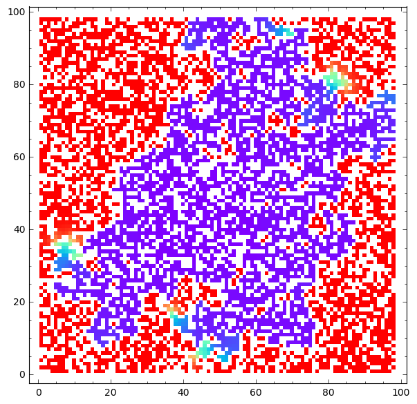
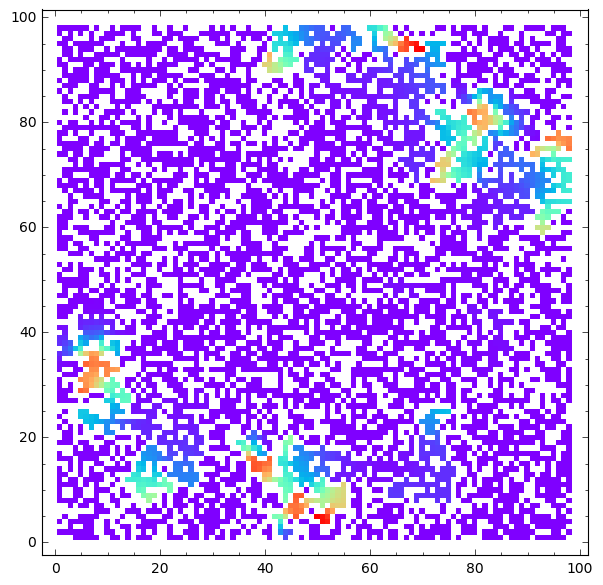
matrix_plot(u*wall,origin='lower',cmap='rainbow',figsize=8 ).show()
matrix_plot(v*wall,origin='lower',cmap='rainbow',figsize=8 ).show()

dt,dt_dyn 0.0520155006191845 0.0200000000000000
sps= 50 dt= 0.0200000000000000 Nsteps= 2500
Saved  50  from  2500

import pylab
@interact
def _(ti=slider(range(len(Tlst)))):
    print r"t=",dt*ti
    pu =  matrix_plot(Tlst[ti]*wall,origin='lower',cmap='rainbow', figsize=(4,4) )
    pv =  matrix_plot(Tvlst[ti]*wall,origin='lower',cmap='rainbow',figsize=(4,4) )
    pu.show()
    pv.show()

Failed to display Jupyter Widget of type sage_interactive.

If you're reading this message in the Jupyter Notebook or JupyterLab Notebook, it may mean that the widgets JavaScript is still loading. If this message persists, it likely means that the widgets JavaScript library is either not installed or not enabled. See the Jupyter Widgets Documentation for setup instructions.

If you're reading this message in another frontend (for example, a static rendering on GitHub or NBViewer), it may mean that your frontend doesn't currently support widgets.

wall = np.ones_like(u)
wall[np.logical_not(m)]=np.nan
anim = animate([matrix_plot(u*wall,origin='lower',cmap='rainbow',figsize=(4,4) ,vmin=0,vmax=1.01) for u in Tlst[::1]])
anim.show()

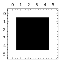
Laplace operator with the reflected wall

import numpy as np
N=6
m = np.ones((N,N),dtype=np.bool)
m[0,:]=False
m[N-1,:]=False
m[:,0]=False
m[:,N-1]=False
show(m)
matrix_plot(m,figsize=3)

$$\newcommand{\Bold}[1]{\mathbf{#1}}\begin{array}{l} \verb|[[False|\phantom{\verb!x!}\verb|False|\phantom{\verb!x!}\verb|False|\phantom{\verb!x!}\verb|False|\phantom{\verb!x!}\verb|False|\phantom{\verb!x!}\verb|False]|\\ \phantom{\verb!x!}\verb|[False|\phantom{\verb!xx!}\verb|True|\phantom{\verb!xx!}\verb|True|\phantom{\verb!xx!}\verb|True|\phantom{\verb!xx!}\verb|True|\phantom{\verb!x!}\verb|False]|\\ \phantom{\verb!x!}\verb|[False|\phantom{\verb!xx!}\verb|True|\phantom{\verb!xx!}\verb|True|\phantom{\verb!xx!}\verb|True|\phantom{\verb!xx!}\verb|True|\phantom{\verb!x!}\verb|False]|\\ \phantom{\verb!x!}\verb|[False|\phantom{\verb!xx!}\verb|True|\phantom{\verb!xx!}\verb|True|\phantom{\verb!xx!}\verb|True|\phantom{\verb!xx!}\verb|True|\phantom{\verb!x!}\verb|False]|\\ \phantom{\verb!x!}\verb|[False|\phantom{\verb!xx!}\verb|True|\phantom{\verb!xx!}\verb|True|\phantom{\verb!xx!}\verb|True|\phantom{\verb!xx!}\verb|True|\phantom{\verb!x!}\verb|False]|\\ \phantom{\verb!x!}\verb|[False|\phantom{\verb!x!}\verb|False|\phantom{\verb!x!}\verb|False|\phantom{\verb!x!}\verb|False|\phantom{\verb!x!}\verb|False|\phantom{\verb!x!}\verb|False]]| \end{array}$$

u = np.random.randn(N,N)
Lap =lambda u: -((u-np.roll(u,1,axis=0))*np.roll(m,1,axis=0)+(u-np.roll(u,-1,axis=0))*np.roll(m,-1,axis=0)+(u-np.roll(u,1,axis=1))*np.roll(m,1,axis=1)+(u-np.roll(u,-1,axis=1))*np.roll(m,-1,axis=1))

print(np.diff(u,2,axis=0)[:,1:-1]+np.diff(u,2,axis=1)[1:-1,:])

[[  0.47679398 -10.81598592  -1.75597319   0.22463036]
 [  3.47819401   3.86554582   3.4607582    6.29143126]
 [  5.46975922  -1.99841518  -6.29319058   0.10127252]
 [ -3.76320216  -2.00004972   0.09766273   4.39892703]]

\[\begin{split}\begin{aligned} \begin{array}{l} \verb|[[-3.13448456|\phantom{xx}\verb|5.18465268|\phantom{xx}\verb|2.24718743|\phantom{xx}\verb|1.5615061|\phantom{x}\verb|]|\\ \phantom{x}\verb|[|\phantom{x}\verb|6.81131198|\phantom{x}\verb|-5.12027386|\phantom{xx}\verb|0.45648868|\phantom{x}\verb|-8.70124209]|\\ \phantom{x}\verb|[|\phantom{x}\verb|0.83522291|\phantom{x}\verb|-2.22075512|\phantom{xx}\verb|4.82439459|\phantom{xx}\verb|5.04618174]|\\ \phantom{x}\verb|[|\phantom{x}\verb|4.44827112|\phantom{x}\verb|-5.28018261|\phantom{x}\verb|-5.41145643|\phantom{x}\verb|-2.22106382]]| \end{array} \end{aligned}\end{split}\]

print(Lap(u))

[[  0.00000000e+00   6.95569230e-03   3.53975387e+00   1.19277480e+00
    4.05144494e-01  -0.00000000e+00]
 [ -5.24724597e-01  -4.09749284e-02  -7.27623206e+00  -5.63198390e-01
   -4.15257753e-01  -1.04503260e+00]
 [ -1.55374939e+00   1.92444461e+00   3.86554582e+00   3.46075820e+00
    3.45042386e+00  -2.84100740e+00]
 [ -2.40269297e+00   3.06706625e+00  -1.99841518e+00  -6.29319058e+00
    8.40887010e-01   7.39614487e-01]
 [ -1.12374597e+00  -1.98448725e+00   2.37829038e-01   4.62887433e-01
    1.26191392e+00  -3.80430201e-01]
 [ -0.00000000e+00   2.90246088e+00   2.23787876e+00   3.65224701e-01
   -2.75658291e+00  -0.00000000e+00]]

\[\begin{split}\begin{aligned} \begin{array}{l} \verb|[[-0.|\phantom{xxxxxxxxxx}\verb|0.42601275|\phantom{x}\verb|-2.51302703|\phantom{x}\verb|-1.25894388|\phantom{xx}\verb|1.13807986|\phantom{x}\verb|-0.|\phantom{xxxxxxxx}\verb|]|\\ \phantom{x}\verb|[|\phantom{x}\verb|0.34635619|\phantom{x}\verb|-2.36211561|\phantom{xx}\verb|2.67162565|\phantom{xx}\verb|0.98824355|\phantom{xx}\verb|1.49902703|\phantom{x}\verb|-1.20055893]|\\ \phantom{x}\verb|[-1.58676378|\phantom{xx}\verb|5.22454821|\phantom{x}\verb|-5.12027386|\phantom{xx}\verb|0.45648868|\phantom{x}\verb|-6.25692915|\phantom{xx}\verb|2.44431293]|\\ \phantom{x}\verb|[-0.21974371|\phantom{xx}\verb|0.61547921|\phantom{x}\verb|-2.22075512|\phantom{xx}\verb|4.82439459|\phantom{xx}\verb|3.49525843|\phantom{x}\verb|-1.55092331]|\\ \phantom{x}\verb|[-1.49169634|\phantom{xx}\verb|2.81477871|\phantom{x}\verb|-3.81338909|\phantom{x}\verb|-1.7187601|\phantom{xx}\verb|-1.09762113|\phantom{xx}\verb|1.90581171]|\\ \phantom{x}\verb|[-0.|\phantom{xxxxxxxxx}\verb|-0.14179607|\phantom{xx}\verb|1.46679352|\phantom{xx}\verb|3.69269634|\phantom{x}\verb|-0.78236901|\phantom{x}\verb|-0.|\phantom{xxxxxxxx}\verb|]]| \end{array} \end{aligned}\end{split}\]