The Lotka-Volterra model with SAGE
Analytical analylsis of Lotka Volterra with computer algebra
The ODE can be analyzed with Sage both analytically as well as numerically. Analytical solution to ODE is difficult to obtain in most realistic cases, but it turs out that it is possible in Lotka Volterra system.
We will use desolve for algebraic manipulations on a system of ODEs and desolve_odeint for its numerical sulution. We will also try to reuse the formulas, so the system definition is given only once. For this purpose we will denote by \(Y(x)\) a Sage function which is required in desolve and use substitution to \(y\) symbolic variable to be used for plotting and numerical operations.
[1]:
var('x a y', domain='real')
Y = function('Y')
rhs =  vector([x-x*Y(x), a*(x*Y(x)-Y(x))])
show(rhs)
We can check for fix-points:
[2]:
var('x y')
solve(list(rhs.subs([Y(x)==y])),  [x,y])
[2]:
[[x == 0, y == 0], [x == 1, y == 1]]
Since we have a system of two autonomous differential equations, we can eliminate time by divigin one equation by another and obtain equation for \(y(x)\).
[3]:
(rhs[1]/rhs[0])
[3]:
-(x*Y(x) - Y(x))*a/(x*Y(x) - x)
[4]:
var('x0 y0')
[4]:
(x0, y0)
If we give a symbolic initial condition to desolve, we will obtain a formula with easier to interpret integration constant.
[5]:
sol = desolve(diff(Y(x),x)==rhs[1]/rhs[0], Y(x), \
              ivar=x, ics=(x0,y0))
[6]:
phase_curve = (a*sol.subs(Y(x)==y)).simplify()
var('alpha')
show( phase_curve.subs([a==alpha,Y(x)==y]) )
[7]:
print(phase_curve)
-y + log(y) == a*x - a*x0 - a*log(x) + a*log(x0) - y0 + log(y0)
[8]:
phase_curve.subs(a==1).show()
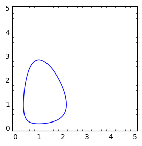
Now we can plot the phase curve for arbitrary initial condition and parameter \(\alpha\)
[9]:
implicit_plot(phase_curve.subs(a==2.1,x0==1,y0==.2),(x,0,5),(y,0,5),figsize=4)
[9]:
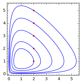
[10]:
a_ = 1
p = Graphics()
x0_ = 2.0
for y0_ in srange(1,6,1):

    p += implicit_plot(phase_curve.subs(a==a_,x0==x0_,y0==y0_),(x,0,5.5),(y,0,5.5),legend_label='y(x=1)=%0.1f'%y0_,plot_points=400)
    p += point((x0_,y0_),color='red',size=15)
p.show(figsize=4)
p.save('lotka_phase.png',figsize=4)
[11]:
phase_curve = -y + log(y) == a*x - a*x0 - a*log(x) + a*log(x0) - y0 + log(y0)

@interact
def _(a_=slider(1e-2,2,0.1,default=1.0),
      x0_=slider(1e-3,4,0.04,default=1),
      y0_=slider(1e-3,2,0.04,default=1.2)):
    p = implicit_plot(phase_curve.subs(a==a_,x0==x0_,y0==y0_),(x,0,5),(y,0,5))
    p += point((x0_,y0_),color='red',size=15,legend_label='ic')
    p.show(figsize=4)
Numerical solutions of Lotka Volterra
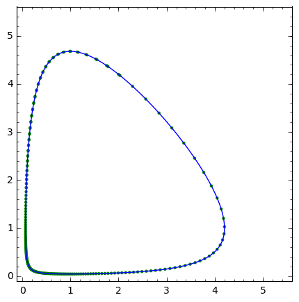
We can use desolve_odeint in order to obtain numerical solution to the system with a given initial condition. It will allow to investingate the time dependence of those ODEs.
We can plot the solution \((x(t),y(t))\) as a parametric curve on a phase plane and compate it with analytical solution obtained in the previous section.
[12]:
a_ = 1.21
x0_ = 2.0
y0_ = 4.2

T = srange(0,9,0.04)
sol = desolve_odeint(rhs.subs([a==a_,Y(x)==y]), [x0_, y0_],T,[x,y])
p = points(sol,color='green')
p += implicit_plot(phase_curve.subs(a==a_,x0==x0_,y0==y0_),(x,0,5.5),(y,0,5.5),legend_label='y(x=1)=%0.1f'%y0_,plot_points=400)

p.show(figsize=6)
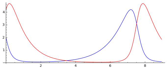
We can also plot numerical solution as a function of time:
[13]:
plt_t = line(zip(T,sol[:,0]))+line(zip(T,sol[:,1]),color='red')
plt_t.show(figsize=(7,3))
[ ]:
phase_curve = -y + log(y) == a*x - a*x0 - a*log(x) + a*log(x0) - y0 + log(y0)
x0_ = 1.0
y0_ = 4.2
a_ = 1.0
Tmax = 20
T = srange(0,Tmax,0.01)

sol = desolve_odeint(rhs.subs([a==a_,Y(x)==y]), [x0_, y0_],T,[x,y])

@interact
def plot_lotka(ith_t=slider(0,len(T),1)):
    i = (ith_t)
    p = implicit_plot(phase_curve.subs(a==a_,x0==x0_,y0==y0_),(x,0,5),(y,0,5),
                     figsize=(16,6))
    p += point((x0_,y0_),color='green',size=50,legend_label='ic')
    p += point(sol[i],color='red',size=50,title='t=%0.3f'%T[i])

    p += plot_vector_field(rhs.subs([a==1.0,Y(x)==y]).normalized(),(x,0,5),(y,0,5))

    p_t = point((T[i],sol[i,0]),color='blue',size=50,figsize=(6,3))
    p_t += point((T[i],sol[i,1]),size=50,color='red')
    p_t += point((T[0],sol[0,0]),color='blue',size=100)

    p_t += line(zip(T,sol[:,0]))+line(zip(T,sol[:,1]),color='green')


    show(graphics_array([[p,p_t]]),figsize=[10,4])
[15]:
phase_curve = -y + log(y) == a*x - a*x0 - a*log(x) + a*log(x0) - y0 + log(y0)
x0_ = 1.0
y0_ = 4.2
a_ = 1.0
Tmax = 16.5
T = srange(0,Tmax,0.01)

sol = desolve_odeint(rhs.subs([a==a_,Y(x)==y]), [x0_, y0_],T,[x,y])

def plot_lotka(ith_t):
    i = (ith_t)
    p = implicit_plot(phase_curve.subs(a==a_,x0==x0_,y0==y0_),(x,0,5),(y,0,5),
                     figsize=(16,6))
    p += point((x0_,y0_),color='green',size=50,legend_label='ic')
    p += point(sol[i],color='red',size=50,title='t=%0.3f'%T[i])
    p += plot_vector_field(rhs.subs([a==1.0,Y(x)==y]),(x,0,5),(y,0,5))
    p_t = point((T[i],sol[i,0]),color='blue',size=50,figsize=(6,3))
    p_t += point((T[i],sol[i,1]),size=50,color='red')
    p_t += point((T[0],sol[0,0]),color='blue',size=100)

    p_t += line(zip(T,sol[:,0]))+line(zip(T,sol[:,1]),color='green')


    return (graphics_array([[p,p_t]]) )
[16]:
animate([plot_lotka(i) for i in range(0,len(T),50)],figsize=[8,2])
[16]:

[ ]:
[ ]:
Period of oscillations
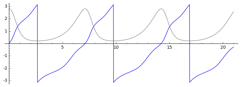
We can numerically determine the period of oscillations. For this purpose we will plot the phase of the point in \((x,y)\) plane:
[17]:
a_ = 1.
x0_ = 2.80
y0_ = 1.
T = srange(0,21,0.01)
sol = desolve_odeint(rhs.subs([a==a_,Y(x)==y]), [x0_, y0_],T,[x,y])

phase_t = arctan2(sol[:,1]-1,sol[:,0]-1)

p = line( zip(T,phase_t))
p += line( zip(T,sol[:,0]),color='gray')
p.show(figsize=(8,3))
We can now calculate time points when phase jumps back by \(-2\pi\) and obtain period od oscillations
[18]:
import numpy as np
phase_jumps = []
for i in np.where(np.diff(phase_t)<0)[0]:
    phi1,phi2 = phase_t[i],phase_t[i+1]+2*np.pi
    eta = (np.pi-phi1)/(phi2-phi1)
    phase_jumps.append(T[i]+eta*(T[i+1]-T[i]))
period = np.mean(np.diff(phase_jumps))
[19]:
plt = line( zip(T,phase_t))
plt += points(zip(phase_jumps,[0]*len(phase_jumps)),color='red',size=20)
plt.show(figsize=(7,2))
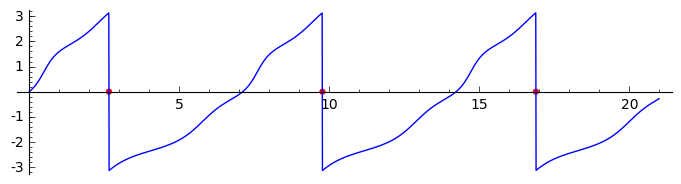
[20]:
phase_jumps
[20]:
[2.6559616060389617, 9.7694250720849354, 16.882901862346589]
[21]:
period
[21]:
7.1134701281538142
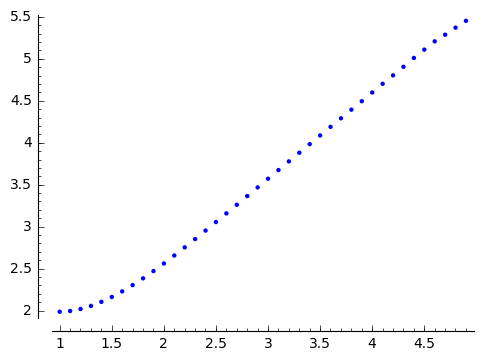
Let us check if and how the period depends on initial condition:
[22]:
import numpy as np
def calculate_period(a_ = 1.,x0_ = 2.0,y0_ = 1.0,dt=0.04, t_end=20):
    """
    Calculate period od a Lotka Volterra model for given parameters
    """
    T = srange(0,t_end,dt)
    sol = desolve_odeint(rhs.subs([a==a_,Y(x)==y]), [x0_, y0_],T,[x,y])
    phase_t = arctan2(sol[:,1]-1,sol[:,0]-1)
    phase_jumps = []
    for i in np.where(np.diff(phase_t)<=0)[0]:
        phi1,phi2 = phase_t[i],phase_t[i+1]+2*np.pi
        eta = (np.pi-phi1)/(phi2-phi1)
        phase_jumps.append(T[i]+eta*(T[i+1]-T[i]))
    if len(phase_jumps)==0:
        period = 0
    else:
        period = np.mean(np.diff(phase_jumps))
    return period
[23]:
point( [(x0_,calculate_period(a_=10.,x0_ = x0_,dt = 1e-2,t_end=10)) for x0_ in srange(1+1e-3,5,0.1)],figsize=5)
[23]:
[ ]: