Introduction to the kinetics of chemical reactions

Kinetics deals with the prediction of time-changes of concentrations of substracts and products during chemical reactions, analysis of rates , influence of various elements on the rate of reactions, and so on.

In chemical reactions, one can observe the change of one or several substances (substrats, reactants) into one or several other substances (products). In modeling of kinetics of reactions one has to construct differential equations for change of concetrations of reaction components (compounds). The construction of evolution equations is based on the Law of Mass Action:

1. the rate of a chemical reaction depends on the product of concentrations of the reactants

2. when a chemical reaction reaches equilibrium, the concentrations of the chemicals involved bear a constant relation to each other, which is described by an equilibrium constant.

It is also called the law of Guldberg and Waage - introduced in 1864 by Norwegian chemist and mathematician, respectively.

It is a fundamental law for chemical kinetics. Based on this, the Swedish chemist Svante Arrhenius deduced a formula for the effect of temperature on the reaction rate constant. The Law of Mass Action describes how the velocity of a reaction depends on the molecular concentrations of the reactants and states that when a chemical reaction reaches equilibrium, the concentrations of the chemicals involved bear a constant relation to each other, which is described by an equilibrium constant.

How to construct equations for kinetics of chemical reactions? Let us note that during the reaction, some substances disappear and some substances appear. It resembles the birth and death process known in population dynamics. Therefore we can use methods we have learned previously. To show it, let us consider the reaction:

\[A + X \overset{ k_1} {\underset {k_2} \longleftrightarrow} B\]

There are two molecules, \(A\) and \(X\), which associate with the rate \(k_1\) forming the molecule \(B\). The molecule \(B\) can dissociate with the rate \(k_2\) into two molecules \(A\) and \(X\). We denote the concentrations of substances by small letters:

\[[A]=a, \quad [X]=x, \quad [B]=b\]

where i.e. \([A]\) denotes concentration of the molecules \(A\). In the population dynamics, it correponds to the function \(N=N(t)\). The rate of change of some function is determined by its derivative. We remind that:

1. if the function increases its derivative is positive

2. if the function decreases its derivative is negative.

In this way, the concentration change of \(A\) is characterized by the derivative:

\[\frac{d a}{dt}\]

According to the Law of Mass Action, it is proportional to the product of concentrations of substances participated in the reaction. If the concentration of a given substance grows then the product is with the sign \("+"\) and if it decreases then it is with the sign \("-"\). Accordingly,

\[\frac{d a}{dt} = -k_1 a x + k_2 b, \quad \quad \frac{d x}{dt} = -k_1 a x + k_2 b, \quad \quad \frac{d b}{dt} = k_1 a x - k_2 b\]

From the form of these equations we note that in the left hand sides the unit is \([1/second]\) because of the derivative with respect to time \(t\). In the right hand sides, the rates must have the same unit \([1/second]\).

Let us consider in detail the first equation. The change of concentration of \(A\) is caused by two processes:

A1. In the left side, for the forward reaction \(A+X\), the substance \(A\) dissapears with the rate \(k_1\). Because there are two substances \(A\) and \(X\) therefore there is a product \(a \cdot x\) of two cencentractions \(a\) and \(x\) which is multiplied by the rate \(k_1\). The expression is with the sign \("-"\) because \(A\) disappears. Finally, the derivative is negative, i.e. we write:

\[-k_1 a x\]

A2. In the rigt side, for the backward reaction, there is only one substance \(B\) which dissociates into two molecules \(A\) and \(X\). The new molecule \(A\) appears with the rate \(k_2\). Because \(A\) is created, the sign is \("+"\) and we write:

\[k_2 b\]

In a similar way, we obtain two other equations.

Autocatalytic reactions

In autocatalytic reaction one of the substrat functions as a catalyst and is also a product. In other words, autocatalytic reactions are those in which at least one of the products is a reactant. Autocatalysis plays an important role in many living processes, e.g. in transcription of rRNA.

Example 1

A simple example of such a reaction is:

\[A + Y \overset{ k_1} {\underset {k_2} \longleftrightarrow} 2Y\]

or equivalently

\[A + Y \overset{ k_1} {\underset {k_2} \longleftrightarrow} Y+Y\]

with reaction rates \(k_1\) i \(k_2\). Let us assume that the concentration \(a\) of the substance \(A\) is fixed at the constant value. It means that \(da/dt=0\). In turn, the concentration \(y\) of the reactant \(Y\) changes in time. Under these conditions the evolution equation reads

\[\frac{dy}{dt}= k_1 a \cdot y - k_2 y \cdot y = k_1 a y - k_2 y^2\]

Lat us attention that there is a product \(y \cdot y\) because in the backward reaction we have two “substances” \(Y+Y\).

We rewrite it to the form

\[\frac{dy}{dt}= k_1 a y [1 - \frac{k_2}{k_1 a} y]\]

In this equation, all parameters are positive. Note that it is similar to the Verhulst equation. Indeed, if we introduce new variables:

\[x= \frac{k_2}{k_1 a} y, \quad \quad s= k_1 a t\]

then in these new variables the differential equation transforms to the form:

\[\frac{dx}{ds}= x [1 - x], \quad x=x(s), \quad x(0) = x_0\]

It is exactly the rescaled Verhulst equation! Therefore it has exacly the same properties as the Verhulst equation.

Experiment with Sage!

Scaling can be done wit the help of Sage. The most straightforward possibility is to define derivative as independent symbolic variables and scale them appropriately.

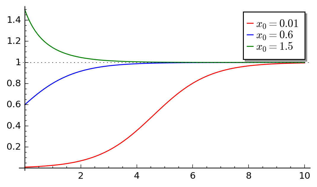
Time evolution of autocatalytic model for different initial conditions.

In the above figure, we depict time evolution of the rescaled concentration \(x = x(s)\) for three selected initial conditions. As it follows from the analysisi for the Verhulst model, there is one stable stationary state d \(x=1\) and one unstable state \(x=0\). The shape of \(x(s)\) for the initial concentration \(x_0=0.01\) is sigmoid. We observe that the speed of the reaction increases with time and the concentration of the product increases and next it decreases because of smaller concentration of substrat. For long time, there is a saturation in concentration of \(Y\).

Experiment with Sage!

Interact with the code to see how does the concentration behaviour depends on initial condition:

Example 2

Let us consider the second example of the autocatalytic reaction:

\[A + Y \overset{ k_1} {\underset {k_2} \longleftrightarrow} 2Y\]

\[B + Y \overset{ k_3} { \rightarrow} C\]

We assume that the concentrations of substances \(A\) and \(B\) is kept constant and it means that \(da/dt = db/dt = 0\). The concentration of \(Y\) changes according to the equation:

\[\frac{dy}{dt} = k_1 a y -k_2 y y - k_3 b y = r y - k_2 y^2\]

where

\[r = k_1 a - k_3 b\]

The form of this equation is similar to the equation for the previous autocatalytic reaction. However, one can note an essential difference, namely, the parameter \(r\) can take positive or negative values!

1. If

\[k_1 a \gt k_3 b \quad \quad \mbox{i.e.} \quad \quad r \gt 0\]

then it is the same case as for the provious reaction (the Verhulst model).

2. If

\[k_1 a \lt k_3 b \quad \quad \mbox{i.e. } \quad \quad r \lt 0\]

then the parameter \(r\) takes negative values and we can rewrite the differential equation as:

(1)\[\frac{dy}{dt} = - r_0 y - k_2 y^2 = f(y), \quad \quad r_0 = |k_1 a - k_3 b| \gt 0, \quad k_2 \gt 0\]

This equation exhibits a radically different solution than the Verhulst one. There is only one stationary state \(f(y) = 0\) and hence \(y=0\). In order to determine its stability, we calculate the derivative \(f'(y) = -r_0 -2k_2 y\) and for the state \(y=0\) one gets \(\lambda = f'(0) = -r_0 < 0\). It follows that \(y=0\) is an asymptotically stable stationary state. So, the substance dissapers and the reason is the relation (b): the rate of the first reaction is too slow in order to compensate decay of \(Y\) caused by the second reaction.

Without loosing generality we can assume that in eq (1) \(k_2=1\). Then we can solve the ODE:

(2)\[\frac{dy}{dt} = r y - y^2\]

Experiment with Sage!

Use Sage to solve analytically ODE (2)

This ODE has a solution for initial condition \(y(0)=y_0\):

\[y\left(t\right) = \frac{r y_{0} e^{r t}}{y_{0} {\left(e^{r t} - 1\right)} + r}\]

Experiment with Sage!

Now we can investigate how solutions for different initial concentrations depend on the parameter \(r\in(-1,1)\).

• start with \(r=1\) - there will be a Vehulst solution again.

• decrease \(r\) to some positive value, the stable solution will change but still will be positive.

• go with \(r\) below zero - the only stable state will be \(x=0\)

Enzyme reactions

Enzymes are catalysts and increase the speed of a chemical reaction without themselves undergoing any permanent chemical change. They are neither used up in the reaction nor do they appear as reaction products. Enzymes are responsible for bringing about almost all of the chemical reactions in living organisms. Without enzymes, these reactions take place at a rate far too slow for the pace of metabolism. Catalysis is the acceleration of a chemical reaction by some substance which itself undergoes no permanent chemical change.

The basic enzymatic reaction is

\[E + S \, \overset{k_f}{\underset{k_r}\Longleftrightarrow} \, ES \, \overset{k_3} {\Longrightarrow} \, E + P\]

where \(E\) represents the enzyme catalyzing the reaction, \(S\) is the substrate being changed, \(ES\) is the complex and \(P\) the product of the reaction.

In 1913, the German biochemist Leonor Michaelis and Canadian physician Maud Menten proposed this model and now it is a basic model of the enzyme kinetics. Applying the Law of Mass Action one obtains the following set of four equations:

(3)\[\begin{split}\begin{aligned} \begin{array}{cccccccc} \displaystyle\frac{ds}{dt} & = & - & k_f e s & + & k_r c & \\ \displaystyle\frac{de}{dt} & = & - & k_f e s & + & k_r c & + & k_3 c \\ \displaystyle\frac{dc}{dt} & = & + & k_f e s & - & k_r c & - & k_3 c \\ \displaystyle\frac{dp}{dt} & = & & & + & k_3 c \end{array} \end{aligned}\end{split}\]

where the small leters denote concentrations of the corresponding substances \(s=s(t), e=e(t), p=p(t)\) and \(c=c(t)\) is the concentration of the comples \(ES\).

Let us impose initial conditions:

\[s(0)= s_0, \quad \quad e(0)=e_0, \quad \quad c(0)=0, \quad \quad p(0)=0\]

These conditions should be obvious: at some initial time, there is non-zero concentration of the substrat \(S\) and enzyme \(E\). There is no complex \(ES\) and there is no product \(P\). They appear in the later time as a result of the reaction.

Below we present a computer program which solves this set of 4 differential equations. Without a computer, it would be difficult to visualise the solutions.

We can use Sage to solve numerically the system MM_min

var('s e c p') ## it is numerical solution of the above set of 4 differential equations
kf,kr,k3 = 5,0.5,1
T = srange(0,5,0.01)
sol = desolve_odeint(\
 vector([-kf*e*s+kr*c,-kf*e*s+kr*c+k3*c, kf*e*s-kr*c-k3*c,k3*c]),\
 [1,0.8,0,0],T,[s,e,c,p])

Time evolution of the substrate, the enzyme, the complex [ES], and the product.

Theoretical analysis a’la Michaelis-Menten

The set of 4 non-linear differential equations seems to be very complicated. However, its specific structure allows to perform analysis to obtain relevant information of the reaction

1. Let us note that the last differential equation can be integrated:

\[p(t) = p(0) + k_3 \int_{0}^t c(\tau) d\tau = k_3 \int_{ 0}^t c(\tau) d\tau\]

If we know time evolution of the complex \(ES\), i.e. \(c(t)\), from this equation we know how the concentration \(p(t)\) of the product \(P\) evolves.

2. Enzyme is a catalyst and therefore its total concentration is constant in time. It is seen when we add both sides of the second and third eqautions:

\[\frac{de}{dt} + \frac{dc}{dt} =0, \quad \quad \mbox{hence it follows that} \quad \quad e(t) + c(t) = const. = e(0) + c(0) = e_0\]

From this relation we get:

\[e(t) = e_0 - c(t)\]

3. From the above considerations in (1) and (2) it follows that it is sufficient to consider only two eqautions:

\[\begin{split}\begin{aligned} \begin{array}{cccccccc} \displaystyle\frac{ds}{dt} & = & - & k_f s [e_0 - c] & + & k_r c &\\ \displaystyle\frac{dc}{dt} & = & + & k_f s [e_0-c] & - & ( k_r + k_3) c \end{array} \end{aligned}\end{split}\]

Let us now rescale these equations to reduce a number of parameters \(k_f, k_r, k_3, e_0\). We define new variables and rescaled parameters:

\[x= \frac{s}{s_0}, \quad y=\frac{c}{e_0}, \quad \tau = k_f e_0 t, \quad \lambda = \frac{k_3}{k_f s_0}, \quad K= \frac{k_r + k_3}{k_f s_0}, \quad \epsilon =\frac{e_0}{s_0}\]

In the new variables, the set of two differential equations assumes the form :

\[\begin{split}\begin{aligned} \begin{array}{cccccccc} \frac{dx}{d\tau} & =& - x + (x+K-\lambda) y, \quad \quad x(0) = 1 \\ \epsilon \frac{dy}{d\tau} & =& x - (x+K) y, \quad \quad y(0) = 0 \end{array} \end{aligned}\end{split}\]

Let us note that \(K - \lambda = k_r/k_f s_0 \gt 0\).

The time behavior of the substrat \(x(\tau)\) and complex \(y(\tau)\), which is presented above as a result of numerical solution, can also be obtained by heuristic considerations. Let us do it:

1. For short time \(\tau\), the concentration \(y(\tau) \approx 0\) because \(y(0)=0\). In turn, \(dx/d\tau \approx -x \lt 0\) because the second term with \(y\) can be neglected. If \(dx/d\tau \lt 0\) then it means that \(x(\tau)\) decreases from the initial value \(x(0)=1\).

2. For small values of \(\tau\), the term \(\epsilon dy/d\tau \approx x \gt 0\) because the second term (this with \(y\)) can be neglected. It means that \(y(\tau)\) increases from the initial value \(y(0)=0\). The concentration of the complex increases as long as the right hand side of the equation for \(y\) is positive. It is zero for such time \(\tau_1\) for which

\[x(\tau_1) - [x(\tau_1) + K] y(\tau_1)=0\]

or if

\[y(\tau_1) = \frac{x(\tau_1)}{x(\tau_1) + K}\]

3. For this instant \(\tau_1\), the derivative \(dy/ d \tau =0\). In turn, \(dx/ d \tau = -\lambda x/[x+K] \lt 0\) (we inserted \(y(\tau_1)\) to the first equation for \(x\)). It means that \(x(\tau)\) decreases and is smaller and smaller approaching zero. For time \(\tau>\tau_1\) the derivative of \(y\) changes the sign, \(dy/ d\tau \lt 0\), and the function \(y(\tau)\) starts to decrease to zero. It is seen in the equation for \(y\) :

\[\epsilon \frac{dy}{d\tau} \approx -K y \lt 0 \quad \mbox{because } \quad x(\tau) \to 0 \quad \mbox{for long time}.\]

In this way, one can obtain qualitative properties of the system of two equations for \(s(t) \propto x(\tau)\) and \(c(t) \propto y(\tau)\). Using the conservation law \(e(t) + c(t) = const. = e(0) + c(0) = e_0\), we can reconstruct evloution of the enzyme concentration \(e(t)\). In turn, the time dependence of the product can be obtained from the equation

\[p(t) = k_3 \int_{ 0}^t c(\tau) d\tau\]

Let us remember about the geometric interpretation of the integral: it is area between the function \(c(t)\) and the horizontal axis. Bacause \(c(t) > 0\), this area increases when the upper limit of integration increases. So, we conclude that the function \(p(t)\) increases when \(t\) increases. Bacuse \(c(t)\) tends to zero when \(t \to \infty\), the area \(p(t)\) tends to a constant value as \(t \to \infty\). Summing up, \(p(t)\) is a monotonically increasing function from 0 for \(t=0\) to a constant value for \(t \to \infty\).

The quasi-steady state approximation

It seems that the simplest case for analysis is when the parameter \(\epsilon = e_0/s_0 \lt \lt 1\). Then in the left hand side of the second equation we can put zero, i.e.,

\[\begin{split}\begin{aligned} \begin{array}{cccccccc}\displaystyle\frac{dx}{d\tau} & =& - x + (x+K-\lambda) y, \\ 0 & =& x - (x+K) y \quad \quad \mbox{hence} \quad \quad y \approx \frac{x}{x+K} \end{array} \end{aligned}\end{split}\]

Inserting the expression \(y\) to the first eqaution we obtain the equation for \(x\), i.e. for substrate:

\[\frac{dx}{d\tau} = - \frac{\lambda x}{x+K}\]

Let us not that the right hand side of this equation is always negative. Therefore \(x=x(\tau)\) is decreasing function of time. It is fully in agrement with the exact numerical solution depicted above. From the mathematical point of view, the used approxamation \(\epsilon = e_0/s_0 \lt \lt 1\) belongs to non-trivial problems of derivative with a small parameter. We leave improved version of analysis for mathematicans and and we will proceed as non-mathematicians. If \(\epsilon = e_0/s_0 \lt \lt 1\) it means that changes of \(y(\tau)\) are slow because its derivative is small. In other words, this degree of freedom is close to the stationary state (which is approached for \(t \to \infty\)). This regime is called the quasi-steady state hypothesis.

Excercises

A1. Find statinary state of the system \((x(\tau), y(\tau))\) and thirs stability.

A2. Check numerically for what values of \(\epsilon\) the quasi-seady state hypothesis is acceptable.

A3. Evaluate the relation for the initial concentration of enzyme and substrate for the coretness of quasisteady state approximation.

Rate of the enzymatic reaction

Finally, let us investigate the rate of formation of the product \(p\). It is determined by the forth equation for the kinetics:

\[\frac{dp}{dt}= k_3 c\]

We assume that the concentration \(c\) of the complex is given within the steady-state hypothesis:

\[c= e_0 y = e_0 \frac{x}{x+K} = e_0 \frac{s/s_0}{s/s_0 +K}\]

So, the rate for formation of the product takes the form

\[v= \frac{dp}{dt} = V_{max} \frac{s}{s+K_m}\]

where

\[V_{max} = k_3 e_0, \quad \quad \quad K_m=\frac{k_r +k_3}{k_f}\]

The parameter \(K_m\) is called the Michaelis constant. The dependence of \(v\) on \(s\) is shown below. When \(s \to \infty\) the rate \(p \to V_{max}\). So, the parametr \(V_{max}\) is the maximal rate achieved by the system. Now, let us calculate the concentration of the substrate \(s=s_h\) at which the rate \(v\) is at half-maximum:

\[\frac{1}{2} V_{max} = V_{max} \frac{s_h}{s_h+K_m} \quad \quad \mbox{hence} \quad \quad s_h = K_m\]

In this way we can identify the meaning of the Michaelis constant: > \(K_m\) is the concentration of substracte \(s\) at which the reaction rate \(v\) takes its half of the maximal value.

The rate of production of the product in Michaelis-Menten kinetics as a function of a substrate concentration.

On can conclude that given en enzyme concentration there is a saturation effect, where adding mode substrate will not give better product growth rate. For parameters as in figures :fig:`MM_ss_1` and :fig:`MM_ss_2` the production was at 75% of its maximum value at the beginning of the reaction course, as we has \(K_m=0.3\) and initial concentration of the substrate equal to one. However, if we start with higher concentration of substrate, then it will stay for relatively long time in the regime of maximum production rate. We depict this situation in figure below.

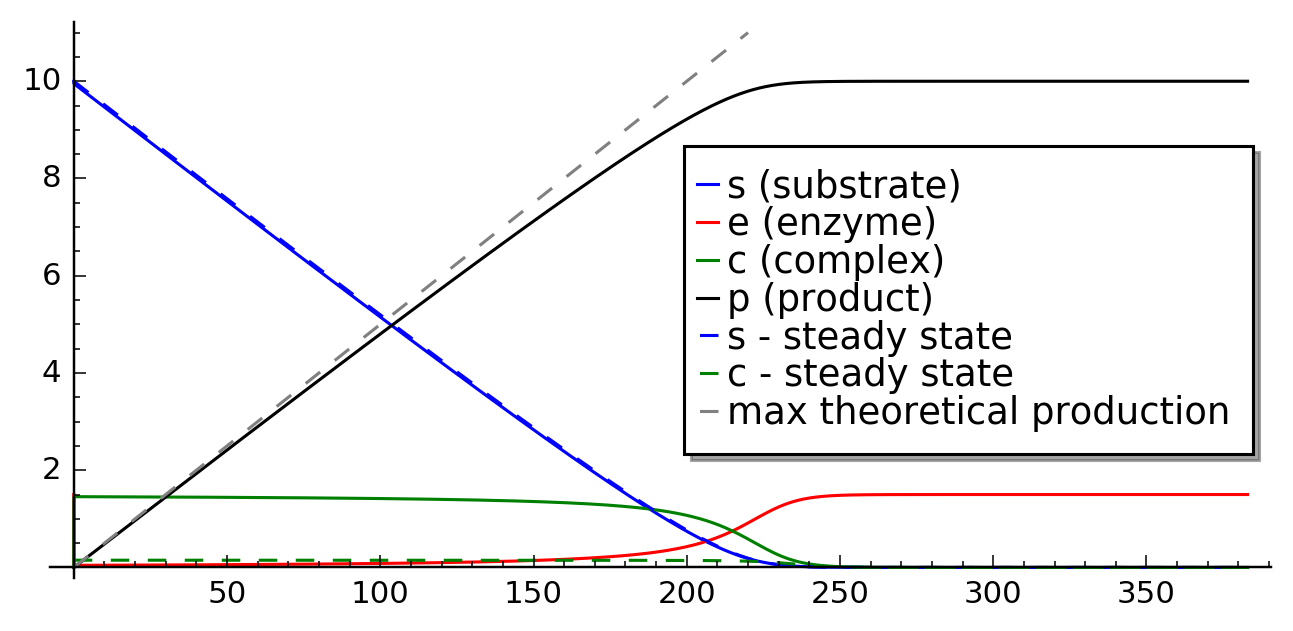
Enzymatic reaction in conditions of maximum enzyme production.

Experiment with Sage!

Below you can find code solving both 4 dimensional kinetic equations as well as the quasi-steaty approximation.

Excercises

1. There is a sequence of chemical reactions:

\[X \overset{ k_1} {\underset {k_2} \longleftrightarrow} A, \quad \quad B \overset{ k_3} { \rightarrow} Y, \quad \quad 2X + Y \overset{ k_4} { \rightarrow}3X\]

B1. Write differential equations for the change of concentrations for \(X\) oraz \(Y\). Assume that the concentrations of \(A\) and \(B\) are constant.

B2. Write equations in the dimensionless form.

B3. Determine stationary states and their stability.

2. There is a sequence of chemical reactions:

\[A \overset{ k_1} {\rightarrow} X, \quad \quad B + X \overset{ k_2} { \rightarrow} Y + D, \quad \quad 2X + Y \overset{ k_3} { \rightarrow}3X, \quad \quad X \overset{ k_4} { \rightarrow} E\]

Assume that the concentrations of \(A, B, D\) and \(E\) are fixed and do not change in time. Do the same as in the previous problem I.