Reaction-diffusion equations

Up to now, we have analysed models of population dynamics and kinetics of chemical reactions without spread in space or area. We have been interested in behavior of the system in time and not in space. It means that modeling is based on ordinary differential equations (derivatives are with repect to time. Changes in space are described by derivatives with respect to coordinates. The we obtain partial differential equations. Mathematical analysis of such equations is much more difficult. Today, an alternative is numerical analysis with the help of computers.

Example: diffusion

If we put a drop of dye into water in a glass, we can observe spread of color and the blop will increases in time. After some time water in glass will be colorful. This process of spread of dye is called diffusion. Particle of dye in water moves in a very irregular way. This molecular motion is called Brownian motion and the particle of dye are named Brownian particles. Brownian particles suspended in fluid collides with particles of fluid and the position of the Brownian particle fluctuates in a chaotic (random) way.

In the mathematical formalism, diffusion can be taken into account by adding the Laplacian to evolution equations:

\[ \begin{align}\begin{aligned}\begin{split}\frac{\partial c(\vec r, t)}{\partial t} = D \Delta c(\vec r, t) = D \left[\frac{\partial^2 }{\partial x^2} + \frac{\partial^2 }{\partial y^2} + \frac{\partial ^2}{\partial z^2} \right] c(\vec r, t) = \\\end{split}\\D \left[\frac{\partial^2 c(\vec r, t)}{\partial x^2} + \frac{\partial^2 c(\vec r, t)}{\partial y^2} + \frac{\partial ^2 c(\vec r, t)}{\partial z^2} \right]\end{aligned}\end{align} \]

where \(c(\vec r, t)\) is the concentration of the dye particles at time \(t\) in the point of space of coordinates \(\vec r = (x, y, z)\). Let us note that the diffusion process is described by the second-order derivatives with respect to the spatial variables. The above equation is named the diffusion equation.

For the initial concentration \(c(x, y, z, 0)\) of particles which all are in the point \((x,y,z)=(0,0,0)\) the solution of the diffusion equation has the form

\[c(x, y, z, t) = [4\pi Dt]^{-3/2} \; exp\left[-\frac{x^2+y^2+z^2}{4Dt}\right]\]

This equations can be solved by e.g. Fourier transform method. It is a Gaussian function of the bell shape. Its half-width is proportional to \(D t\). It means that if time \(t\) increases, the half-with increases and this property describes spread of diffusiong particles.

For the proces only in one dimension, e.g. along the \(OX\) axis, the corresponding diffusion equation has the form

\[\frac{\partial c(x, t)}{\partial t} = D \frac{\partial^2 }{\partial x^2} c(x, t) = D \frac{\partial^2 c(x, t) }{\partial x^2}\]

Its solution reads

\[c(x, t) = [4\pi Dt]^{-1/2} \; exp\left[-\frac{x^2}{4Dt}\right]\]

If we want to take into account the spatial spread of population (or chemical products), we can formulate the following method:

Recipe

One has to add the Laplace operator to evolution equations

If spread is in 2-dimensional region, we should add the term:

\[+ D \left[ \frac{\partial^2 }{\partial x^2} + \frac{\partial^2 }{\partial y^2} \right] c(x, y, t)\]

Solution of the 2-dimensional diffusion equation is the Gaussian function on the form:

\[c(x, y, t) = [4\pi Dt]^{-2/2} \; \exp\left[-\frac{x^2+y^2}{4Dt}\right] =\frac{1}{4\pi Dt} \; \exp\left[-\frac{x^2+y^2}{4Dt}\right]\]

var('x,y,t')
c(x,y,t) = 1/(4*pi*t)*exp(-(x^2+y^2)/(4*t))
plts = [ plot3d(c(x,y,t), (x,-4,4), (y,0,8), rgbcolor=hue(t/2.0)) for t in [0.5,1.0,1.5,2.0]]

@interact
def _(viewer=['tachyon','jmol','canvas3d']):
    show(sum(plts),viewer=viewer)

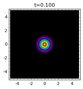
def plt_t(t,**kwargs):
    cmax = c(0,0,t)
    return contour_plot( c(x,y,t) ,(x,-5,5),(y,-5,5),contours=srange(0.01,cmax,cmax/20.0),
                        cmap='spectral',figsize=(3,3),**kwargs)

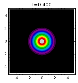
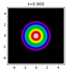
times = [.1,0.4,0.9]
for t in times:
    plt_t(t).show(title="t=%0.3f"%t)

All considered models (Malthus, Verhuslt, chemical reactions, Lotka-Volterra, May, …) can be extended includin spatial chages. For example, if an evolution equation has the form

\[\frac{dN(t)}{dt} = F(N(t))\]

then its generalization with diffusion has the form

\[\frac{\partial N(\vec r, t)}{\partial t} = F(N(\vec r, t) ) + D \Delta N(\vec r, t)\]

where the Laplacian can be taken in 1, 2 or 3 dimensions.

This type of equations are called reaction-diffusion equations

Below, we consider two examples: the Malthus model and the Verhulst model with diffusion.

The Malthus model with migration: The Skellam equation

The standard Malthus model is the simplest model of growth or dacay processes. It is defined by the equation

\[\frac{dN(t)}{dt} = k N(t), \quad k - real\]

If the population can randomly moves on the plane \(XY\) then the extended equation takes the form

\[\frac{dN(x, y, t)}{dt} = k N(x, y, t) + D \left[ \frac{\partial^2 }{\partial x^2} + \frac{\partial^2 }{\partial y^2} \right] N(x, y, t)\]

where now \(N(x, y, t)\) is the concentration (density, i.e. a number of individuals per unit area) in the instant \(t\) in the point on the \(XY\) plane with the coordinates \((x, y)\). It is one of the simplest example of the reaction-diffusion equation. In the literarure, this equation is called the Skellam equation. In 1951, he proposed the model of invasion of the muskrat in Europe. Muskrat (Ondatra zibethica) is a large rodent closely related to rats, mice, voles, hamster and lemmings. Muskrat is also known as a North American aquatic rodent. Muskrats possess wetlands, swamps, and zones close to the lakes, ponds, and streams. In specific parts of the world, muskrats are thought to be pests since they harm waterway dams and feast upon the yields. Individuals chased muskrats in the past just because of their fur and meat. In history, they had been the most trapped animals, for their fur having an economic value.

It is interesting that only 5 muskrats released near Prague in 1905 was the source of rapid expansion year after year. Many millions of muskrats caused a big agriculture and ecological problems. The impact of muskrats on aquatic system is in general negative, especialli in the central Europe. It is a classic example what may happen when animals are transferred into new regions.

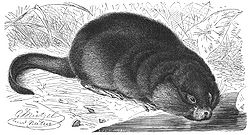
Bisamratte

In this model, we consider only such cases when \(N(x, y, t) \ge 0\). Aditionally, we need:

1. the initial condition \(N(x, y, 0)= N_0(x, y)\)

2. boundary conditions

The above equation can be solved by the substitution

\[N(x, y, t)=e^{kt} c(x, y, t)\]

where $c(x, y, t) is a new unknown function. If we insert it to the reaction-diffusion equation, we see that the new function \(c(x, y, t)\) fulfils the equation

\[\frac{d c(x, y, t)}{dt} = D \left[ \frac{\partial^2 }{\partial x^2} + \frac{\partial^2 }{\partial y^2} \right] c(x, y, t)\]

It is a standard diffusion equation in the 2-dimensional space and its solution is presented in the previous part. So, the function \(N(x, y, t)\) has the form

\[N(x, y, t)=e^{kt} c(x, y, t) = \frac{N_0}{4\pi Dt} \; exp\left[kt -\frac{x^2+y^2}{4Dt}\right]\]

where stała \(N_0=N(0)\) is a concentration of individuals in population at the initial time \(t=0\).

Because \(N(x, y, t)\) is a number of individuals per unit of area, hence

\[\int_{-\infty}^{\;\infty} \;\int_{-\infty}^{\;\infty} N(x, y, t) \,dx \,dy = N(t) = N(0) e^{kt}\]

Let us note that evolution of concentration depends on the coordinates in such a way

\[N(x, y, t)= N(r ,t) = \frac{N_0}{4\pi Dt} \; exp\left[kt -\frac{r^2}{4Dt}\right]\]

where

\[r^2=x^2+y^2\]

is a distance from the origin of the coordinate system.

Analysis of \(N(r, t)\) can be performed with the help of Sage. Below we present graphical presentation.

sage: g(x,t) = (1/(4*pi*t))*exp(t-x^2/(4*t)) sage: @interact sage: def _(t=slider(0.1,5,0.01)): … pr0 = plot( g(x,0.1),(x,0,10),color=’black’ ) … prt = plot( g(x,t),(x,0,10),fill=True ) … (pr0+prt).show(figsize=5)

We observe the following evolution of the population:

1. At initial time the distribution has a fixed form (e.g. for \(t=0.1\)).

2. With time the population spreads and its concentration around \(r=0\) starts to decrease and small time tempo of birth is small.

3. After some time, the concentration in the vicinity \(r=0\) is minimal and next starts to increase (because tempo of birth is greater and greater). At the same time the population spreads in bigger territory.

4. Next, there a moment when the concentration close to \(r=0\) exceeds the initial concentration and the invasion non-stop increases.

The complete analysis of this model can be found in the book:

Nanako Shigesada and Kohkichi Kawasaki, Biological Invasion: Theory and Practice (Oxford University Press, 2001)

Verhulst model with migration: Fisher-Kolmogorov equation

Verhulst model describes time evolution of the population in the situation of limited sustaining resources of the environment:

\[\frac{dn(t)}{dt} = r n(t) \; [1- n(t)]\]

where rescaled concentration \(n(t) = N(t)/K\) and the parameter \(K\) is called the carrying capacity.

This model describes kinetics of two autocatalytic reactions:

\[A + X {\Longleftrightarrow} 2X , \quad \quad \mbox{or } \quad A+X {\Longleftrightarrow} 2X, \quad B+X \rightarrow C\]

If we want to take into account the spatial spread of substances we have to extend the model with the diffusion term:

\[\frac{\partial n(\vec r, t)}{\partial t} = r n(\vec r, t) \;[1- n(\vec r, t)] + D \Delta n(\vec r, t)\]

In the case of population, we should consider 2-dimensional space ( i.e. the Laplacian on the plane) and for chemical reactions - 3-dimensional space. Both realistic cases are complicated from the mathematical point of view. Therefore we make simplification and consider 1-dimensional case od diffusion:

\[\frac{\partial n(x, t)}{\partial t} = r n(x, t) \;[1- n(x, t)] + D \frac{\partial^2 n(x, t)}{\partial x^2}\]

This equation is called the Fisher-Kolmogorov equation.

As usual, we assume that \(n(x, t) \ge 0\). Additionally, we have to impose:

1. the initial distribution of population \(n(x, t= 0)= n_0(x)\)

2. boundary conditions for \(n(\pm\infty, t)\)

Baoundary conditions will be formulated later.

Analysis of the Fisher-Kolmogorov equation

1. Let us notice that the constant functions \(n(x,t) = n_{0} = 0\) and \(n(x, t) = n_{1} = 1\) are solutions of this equation. These are stationary states, the same as in the ordinary Verhulst equation.

2. The equation can be rescaled:

\[\tau = rt, \quad \quad y^2=\frac{r}{D} x^2, \quad \quad n(x,t) \equiv c(y, \tau)\]

The rescaled concentration obeys the equation

\[\frac{\partial c }{\partial \tau} = c [1- c ] + \frac{\partial^2 c}{\partial y^2}, \quad \quad c=c(y, \tau)\]

The functions \(c=0\) and \(c=1\) are stationary solutions.

3. We look for the solutions in the form of waves:

\[c(y, \tau) = U(z), \quad \mbox{where } \quad z=y-v_0 \tau\]

It means that the weve moves into the right direction with the velocity \(v_0\). Frequently we say that the traveling wavefront moves in the right with the speed \(v_0\).

Let us notice that the following eqalities hold:

\[\frac{\partial c }{\partial \tau} = \frac{\partial U}{\partial \tau} = \frac{d U}{d z} \frac{\partial z}{\partial \tau} = -v_0 \frac{d U}{d z}\]

\[\frac{\partial c }{\partial y} = \frac{\partial U }{\partial y} = \frac{d U }{d z} \frac{\partial z }{\partial y} = \frac{d U }{d z}\]

\[\frac{\partial ^2 c }{\partial y^2} = \frac{\partial^2 U }{\partial y^2} = \frac{d ^2U }{d z^2}\]

Hence, the new function \(U(z)\) obeys the ordinary differential equation of the second order:

\[U'' + v_0 U' + U(1-U)=0\]

It is equaivalent to a set of two ordinary differential equations:

\[U'=V = F(U, V), \quad \quad V'=-v_0 - U(1-U) = G(U, V)\]

Now, we can use standard methods and find stationary states:

\[F(U, V) = 0, \quad \quad G(U, V) = 0,\]

As a result we get two sets of stationary solutons:

\[(U_0, V_0) = (0, 0), \quad (U_1, V_1) = (1, 0)\]

1. We determine stability of these states. To this aim, we calculate the Jacobi matrix

\[\begin{split}\begin{aligned} \quad \quad \quad \quad J = \begin{bmatrix}\frac{ \partial F}{\partial U}& \frac{\partial F}{\partial V}\\ \frac{\partial G}{\partial U}& \frac{\partial Gg}{\partial V} \end{bmatrix}= \begin{bmatrix}0, & 1\\ -1+2U, & -v_0 \end{bmatrix} \end{aligned}\end{split}\]

For the stationary states we have:

\[\begin{split}\begin{aligned} J_0= J(0, 0) = \begin{bmatrix}0& 1\\ -1& -v_0 \end{bmatrix}, \quad \quad J_1= J(1, ) = \begin{bmatrix}0& 1\\ 1& -v_0 \end{bmatrix} \end{aligned}\end{split}\]

2. Next, we have to determine eigen-values of the Jacobi matrices \(|J-\lambda I|=0\):

1. for the stationary state \((0, 0)\) one gets:

\[\lambda_{\pm}(0, 0) = (1/2)[-v_0\pm\sqrt{v_0^2-4}]\]

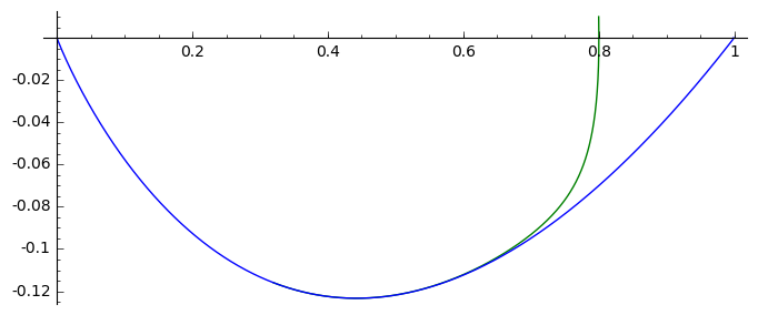
We have to consider two cases: \(v_0 \lt 2\) and \(v_0 \ge 2\). In the first case the eigen-values are complex and their real parts are negative. It means that the phase curve is a spiral which tends to the origin \((0, 0)\). In turn, it means that \(U\) can take negative values (the concentration cannot be negative!). In ceonsequence, we can consider only the second case

\[v_0 \ge 2\]

2. for the stationary state \((1, 0)\) one gets:

\[\lambda_{\pm}(1, 0) = (1/2)[-v_0\pm\sqrt{v_0^2+4}]\]

Because one eigen-value is positive, this state in unstable (it is a saddle point).

F(u,v)=v
G(u,v)= -2*v-u+u^2
T1 = srange(0,5,0.01)
T2 = srange(0,29,0.01)
solo2 = desolve_odeint(vector([F,G]), [0.8, 0.01], T1, [u,v]) # warunek pocz (U, V)
solo3 = desolve_odeint(vector([F,G]), [0.999, 0], T2, [u,v]) # warunek pocz (U, V)
list_plot(solo2.tolist(), plotjoined=True, color='green', figsize=(7,3)) +\
  list_plot(solo3.tolist(), plotjoined=True, figsize=(7,3))

From the above figure it follows that there are initial states close to the state \((1, 0)\), which tend to the state \((0, 0)\). We present it for two initial conditions \((U(0), V(0)) =(0.8, 0.01)\) and \((U(0), V(0)) =(0.999, 0)\). Both trajectories tend to the point \((0, 0)\). In other words, the function \(U(z)\) in the neighbourhood

\(U(z) \approx 1\) is linked with the function \(U(z)=0\). It suggest the boundary conditions:

\[\lim_{z\to -\infty} U(z) = 1, \quad \quad \lim_{z\to \infty} U(z) = 0\]

We remember that in the standard Verhulst equation \(n(t) \to 1\) for \(t\to \infty\). It means that for the fixed value \(y\):

\[\lim_{z\to -\infty} U(z) = \lim_{\tau \to \infty} U(y-v_0 \tau ) = \lim_{\tau \to \infty} c(y, \tau ) = 1\]

and it is consistent with the case without migration.

An exact solution for a particular case

It is one particular case for which the solution of the Fisher-Kolmogorov equation can be presented in an analytical form. For the wave speed

\[v_0 = \frac{5}{\sqrt{6}}\]

the solution reads :

\[c(y, \tau) = \frac{1}{\left\{1+A \exp\left[ (y-v_0 \tau)/\sqrt{6}\right] \right\}^{2}}\]

where the constant \(A\gt 0\) determines the initial concentration profile.

A=1                                              ## określa początkowy profil koncentracji
b=5/sqrt(6)                                      ## prędkość frontu falowego
cs(x,t) = 1/(1+ A*exp(x-b*t)/sqrt(6))^2          ## szczególna, ale analityczna postać frontu koncentracji
@interact
def _(t=slider(0,5,0.2)):
    pr3 = plot( cs(x,0),(x,-10,10),color='black' )
    pr4 = plot( cs(x,t),(x,-10,10),fill=True )
    (pr3+pr4).show(figsize=5)

Failed to display Jupyter Widget of type sage_interactive.

If you're reading this message in the Jupyter Notebook or JupyterLab Notebook, it may mean that the widgets JavaScript is still loading. If this message persists, it likely means that the widgets JavaScript library is either not installed or not enabled. See the Jupyter Widgets Documentation for setup instructions.

If you're reading this message in another frontend (for example, a static rendering on GitHub or NBViewer), it may mean that your frontend doesn't currently support widgets.

Numerical analysis of the Fisher-Kolmogorov equation:

\[\frac{\partial n(x, t)}{\partial t} = r n(x, t) \;[1- n(x, t)] + D \frac{\partial^2 n(x, t)}{\partial x^2}\]

For numerical solution of this equation, we take the simplest discrete verion of the differential equation using the definition of the derivative:

\[\frac{dg(t)}{dt} = B(g(t)) \quad \to \quad g^{i+1} = g^i + dt\; B(g^i)\]

and for the Laplace operator:

\[\frac{d^2 f(x)}{dx^2} \quad \to \quad Lf^k = (dx)^2 \; [f^{k+1} - 2f^k + f^{k-1}]\]

Then the discrete form of Fisher-Kolmogorov equation takes the form:

\[u^{i+1} = u^i + dt \left( r u^i (1-u^i) + D \frac{1}{h^2} Lu^i\right),\]

We assume the periodic boundary conditions by an appropriate choice of the discrete version of the Laplacian. We discretize the space (here the line) and next we fix the time step.

In order obtain solutions of the traveling wave one has to assume small value od the diffusion constant less than \(D\lt 0.001\) in the vicinity of \(r=0\). The length of the system can be incorporated in \(D\), so one can take the length as 1.

import  numpy as np
Dyf = 1.0
r = 1.0
l = 100.0 # dlugosc ukladu
t_end = 50 # czas symulacje
N = 100 # dyskretyzacja przestrzeni
h = l/(N-1)
dt = 0.2/(Dyf*(N-1)**2/l**2) # 0.2 z warunku CFL, krok nie moze byc wiekszy
sps = int(1/dt) # liczba krokow na jednostke czasu
Nsteps=sps*t_end  # calkowita liczba krotkow
print "sps=",sps,"dt=",dt
one = np.identity(N)
L=np.roll(one,-1)+np.roll(one,1)-2*one
L[0,0]=-2.
L[-1,-1]=-2.
L[0,-1]=1.
L[-1,0]=1.
# warunek poczatkowy
u = np.zeros(N)
u[N/2-10:N/2+10]=.1 # small bump
#u[:N/2]=1 # step
Tlst=[]
for i in range(Nsteps):
    if not i%sps:
        Tlst.append(list(u))
    u = u + dt*(r*u*(1-u) + Dyf*(N-1)**2/l**2*L.dot(u))
@interact
def _(ti=slider(range(len(Tlst)))):
    print r"tau=",dt*ti
    p =  list_plot(Tlst[ti],plotjoined=True)
    p += list_plot(Tlst[-1],plotjoined=True,color='red',ymin=0,ymax=1.5)
    p += list_plot(Tlst[0],plotjoined=True,color='gray')
    p.show(figsize=(8,3))

sps= 4 dt= 0.204060810121416

Failed to display Jupyter Widget of type sage_interactive.

If you're reading this message in the Jupyter Notebook or JupyterLab Notebook, it may mean that the widgets JavaScript is still loading. If this message persists, it likely means that the widgets JavaScript library is either not installed or not enabled. See the Jupyter Widgets Documentation for setup instructions.

If you're reading this message in another frontend (for example, a static rendering on GitHub or NBViewer), it may mean that your frontend doesn't currently support widgets.

import numpy as np
Dyf = 1.0
r = 1.0
l = 100.0 # dlugosc ukladu
t_end = 100 # czas symulacje
N = 200 # dyskretyzacja przestrzeni
h = l/(N-1)
dt = 0.052/(Dyf*(N-1)**2/l**2) # 0.2 z warunku CFL, krok nie moze byc wiekszy
sps = int(1/dt) # liczba krokow na jednostke czasu
Nsteps=sps*t_end  # calkowita liczba krotkow
print "sps=",sps,"dt=",dt
one = np.identity(N)
L=np.roll(one,-1)+np.roll(one,1)-2*one
L[0,0]=1.
L[-1,-1]=1.
# warunek poczatkowy
u = np.zeros(N)
#u[:int(N/2]=1 # step
for i in range(1,3):
     u[i] = 1.0 - i/3.0
def essential_boundary_conditions(u):
     u[0] = 1.
     u[-1] = 0.0
Tlst=[]
essential_boundary_conditions(u)
for i in range(Nsteps):
     if not i%sps:
         Tlst.append(list(u))
     u = u + dt*(r*u*(1-u) + Dyf*(N-1)**2/l**2*L.dot(u))
     essential_boundary_conditions(u)
@interact
def _(ti=slider(range(len(Tlst)))):
     print r"t=",dt*ti
     p =  list_plot(Tlst[ti],plotjoined=True)
     p += list_plot(Tlst[-1],plotjoined=True,color='red',ymin=0,ymax=1.5)
     p += list_plot(Tlst[0],plotjoined=True,color='gray')
     p.show(figsize=(8,3))

sps= 76 dt= 0.0131309815408702

Failed to display Jupyter Widget of type sage_interactive.

If you're reading this message in the Jupyter Notebook or JupyterLab Notebook, it may mean that the widgets JavaScript is still loading. If this message persists, it likely means that the widgets JavaScript library is either not installed or not enabled. See the Jupyter Widgets Documentation for setup instructions.

If you're reading this message in another frontend (for example, a static rendering on GitHub or NBViewer), it may mean that your frontend doesn't currently support widgets.

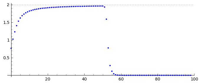
Speed of the wave front

pos_lst = []
for T_ in Tlst:
    for (i,a),b in zip(enumerate(T_),T_[1:]):
        if a>=0.5 and b<=0.5:
            pos_lst.append( i+(a-0.5)/(a-b) )

list_plot( [l/(N-1)*(b-a)/(sps*dt) for a,b in zip(pos_lst,pos_lst[1:])] , figsize=(7,3),gridlines=[[],[2]],ymax=2)