Models of interacting populations: prey-predator

The Lotka-Volterra model

In this model we consider two populations: the population of prey and the population of predators. Prey and predators can be reproduced by the birth process. Population of prey is described by the function \(N=N(t)\) and population of predators - by \(P=P(t)\). As in the Malthus model the rate of change of populations is the birth and death process:

\[\frac{dN}{dt} = a N - b N\]

\[\frac{dP}{dt} = c P - e P\]

where the parameter \(a\) characterizes the birth of prey, \(b\) corresponds to the death process of prey, \(c\) describes the birth process of predators and finally \(e\) corresponds to the death process of predators.

We assume that the death rate \(b\) of prey depends upon the population of predators: If there is a greater number of predators \(P\) then \(b\) should be greater. In the simplest modeling we assume that it is a linear function, i.e.,

\[b \to b_0 P\]

where \(b_0\gt 0\) is a new parameter related to the death rate of prey. Next, we assume that \(C\) depends on the population \(N\) of prey: If there is a greater number of prey then the birth rate of predators is greater, i.e.,

\[c \to c_0 N\]

where \(c_0 \gt 0\) characterizes the birth rate of predators. Under these assumptions, the model reads

\[\frac{dN}{dt} = a N - b_0 P N\]

\[\frac{dP}{dt} = c_0 N P - e P\]

All parameters in this model are positive. This model was introduced by V. Volterra in 1926 to describe population of fish. In 1920 A. J. Lotka considered a similar equation to describe kinetics of some chemical reactions. Therefore this model is called the Lotka-Volterra one. There are 4 parameters. Haw many relevant parameters are in this model? To answer this questions we have tp transform the set of two equations to the dimensionles form. We introduce the following new resclaed variables for populations: b

\[x=\frac{c_0}{e} N, \quad y =\frac{b_0}{a} P\]

and dimensionless time (similarly as in the Verhulst model):

\[\tau = a t\]

In the new variables the Lotka-Volterra set of equations is transformed to the form

\[\dot x= x- x y\]

\[\dot y = \alpha (xy-y)\]

We note that only 1 relevant parameter occurs, i.e., \(\alpha = e/a \gt 0\). It is the ratio of the death rate of predators \(e\) to the birth rate of prey \(a\). The scaling procedure allowed to eliminate irrelevant parameters of the model. There is only one relevant parameter \(\alpha\). In consequence, solutions of the Lotka-Volterra system depens on this parameter and initial conditions \([x(0), y(0)]\).

Stationary states of the system

Stationary states of the system are determined by a set of 2 algebraic equations:

\[f(x, y) = x- x y =0, \quad g(x,y) = \alpha (xy - y) =0,\]

Hence we obtain two pairs of states:

\[(x_1=0, y_1=0) \quad \mbox{or} \quad (x_2=1, y_2 =1)\]

Stability of the stationary states

1. In the first step we have to calculate the Jacobi matrix:

\[\begin{split}\begin{aligned} J = \begin{bmatrix}\frac{ \partial f}{\partial x}& \frac{\partial f}{\partial y}\\ \frac{\partial g}{\partial x}& \frac{\partial g}{\partial y} \end{bmatrix} \end{aligned}\end{split}\]

2. Next, we calculate it for the stationary points:

\[\begin{split}\begin{aligned} J_1= J(0, 0) = \begin{bmatrix}1& 0\\ 0& -\alpha \end{bmatrix}, \quad \quad J_2= J(1, 1) = \begin{bmatrix}0& -1\\ \alpha& 0 \end{bmatrix} \end{aligned}\end{split}\]

3. We have to calculate the eigenvalues of the Jacobi matrix \(|J-\lambda I|=0\):

C1. For \((0, 0)\) we get:

\(\lambda_{01} = 1,\quad \lambda_{02} =- \alpha\).

This state is unstable because one of the eigenvalues is positive \(\lambda_{01} \gt 0\). An arbitrary small perturbation causes the escape from this state.

C2. For \((1, 1)\) we get:

\(\lambda_{11} = i \sqrt{\alpha}, \quad \lambda_{12} = -i\sqrt{\alpha}\).

Two eigenvalues are imaginary. Therefore this state is stable but not asymptotically stable. An arbitrary small perturbation causes the creation of a new time-dependent asymptotic state which is in the vicinity of \((1, 1)\) but does not tends to \((1, 1)\).

Phase curves

We will obtain the phase trajectories or phase curves, i.e. the curves on the plane \((x, y)\). The phase curves are given by the parametric relation \((x(t), y(t))\). To get its form, we devide the second equation by the first equation in the set of two Lotka-Volterra equations. As a result, one has:

\[\frac{dy}{dx}= \frac{\alpha y (x-1)}{x(1-y)}\]

It is a differential equation of the first order. It can be solved by the method of variables separation:

\[\left(\frac{1}{y} - 1\right) \; dy = \alpha \left(1-\frac{1}{x}\right)\; dx\]

The integration of both sides of this equation yields:

\[\mbox{ln} y -y = \alpha (x- \mbox{ln} x) - H_0\]

where \(H_0\) is the integration constant. Its value is determined by initial conditions \((x(0), y(0)\). The minimal value is for the initial conditions \((x(0)=1, y(0)=1)\)> we insert these value to the above equation and get \(H_0 = 1+\alpha\). The explicit dependence of the integration constant on initial condition reads:

\[H_0 = \alpha x_{0} - \alpha \log\left(x_{0}\right) + y_{0} - \log\left(y_{0}\right)\]

In a figure we present few phase curves for selected \(H_0\) corresponding to different initial conditions shown as red dot. . Because the relation between \(y\) and \(x\) is an implicit equation its graphical realization can be obtained by using of SAGE in the following way:

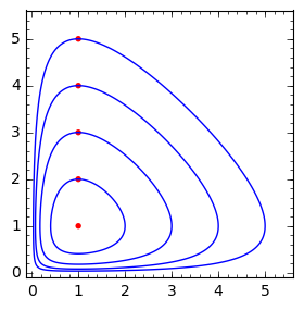
Phase curves of the Lotka-Volterra system. Red dots denote initial condition. Integration constant \(H_0=2.31,2.61,3.21,3.92,4.70\).

Experiment with Sage!

Investigate how parameters: initial condition \(x_0,y_0\) and \(\alpha\) change phase curves of the Lotka-Volterra system.

First, we note that the phase curves are closed. It means that the solutions are periodic (oscillatory) functions of time. Secondly, the increase of \(H_0\) causes the increase of amplitude of oscillations. Below we demonstrate it solving numerically the set of Lotka-Volterra equations.

Time evolution in Lotka-Volterra systems

The time dependence of \(x(t)\) and \(y(t)\) can easily be obtained using the SAGE:

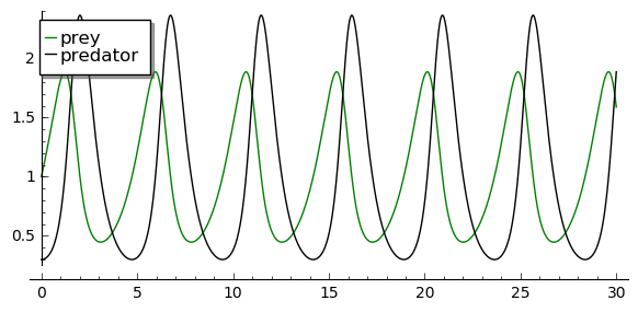
Time evolution in Lotka-Volterra system

Let us note that maxima of \(y(t)\) (population of predators) are delayed to maxima of \(x(t)\) (population of prey). It seems to be obvious: if predators have much food their birth rate grows but in turn it leads to the decrease of the prey number. In consequence the access to food is limited for predators. It causes the lower birth rate for predators and larger growth rate for prey. In turn, food resorces for predators are greater and their growth rate increases. The cycle starts to repeat.

What is the relation between \(H_0\) and the period of oscillations? Below we show the influence of initial conditions (i.e. \(H_0\)) on the oscillations period. We can plot several timeseries with Sage and draw some conclusions.

Experiment with Sage!

Investigate how the initial condition (i.e. integration constant) change phase the frequency of oscillations.

However, it is better to determine the period numerically from the solution and

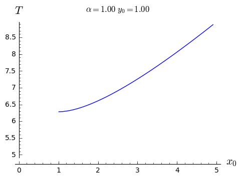
The dependence of oscillation period on initial condition aor a fiven dimensionless paramter.

We conclude that if the phase curve is boarder i.e. \(H_0\) increases, then amplitude and the oscillations period is growssmaller as well.

More realistic: the May model

In the Lotka-Volterra model there is one stable (but not asymptotically) stationary state. When at the intial time \((x(0)=1, y(0)=1)\) then at any time \(x(t)=1\) and \(y(t)=1\) is a solution of the Lotka-Volterra equations. The small perturbations destroy this state and small oscillations appear. Frequently another behavior is observed: If the system is perturbed from sthe stationary state it returns to the previous state. Then we say that the system is structurally stable. This feature is absent in the Lotka-Volterra system. We remind that this system is a modification of the 2-dimenional Malthus model:

\[\frac{dN}{dt} = a N - b N\]

\[\frac{dP}{dt} = c P - e P\]

in which the birth and death processes are modeled in the simplest way. From our experience with other models presented hitherto we can modify the above model in the following way:

1. In the equation for \(N\) we add the part from the Verhulst model and add saturation effects from predations like in the Ludwig model with the Hill function:

\[a=r\left(1-\frac{N}{K}\right), \quad \quad bN = b_0 \,\frac{N}{D+N} \;P\]

2. In the equation for \(P\) we include the Verhulst term:

\[c = c_0 \left(1-\frac{P}{K_0} \right)\]

Therefore in the second equation we obtain

\[c P - e P = c_0 \left(1-\frac{P}{K_0} \right)\;P - e P = (c_0 - e) P - c_0 \frac{P^2}{K_0} = s P \left(1- \frac{P}{K_1} \right)\]

We assume that \(s=c_0-e \gt 0\). The re-scaled parameter \(K_1 = K_0 (1-e/c_0).\)

The parameter \(K_1\) modeling the carrying capacity for predators is proportional to a number of prey \(K_1=h_0 N\) (\(h_0 \gt 0\) is a proportional constant). Finally we get

\[c = s \left(1- h \frac{P}{N}\right)\]

where the new parameter \(h=1/h_0\).

Taking into account the above considerations we arrive at the following set of equations ( (R. May, Models for two interacting populations, in Theoretical Ecology. Principles and Applications, 2nd edition (ed. R. May), 1981, 78-104).

\[\frac{dN}{dt} = r \left(1-\frac{N}{K}\right) \; N- b_0 \frac{N}{D+N} \; P\]

\[\frac{dP}{dt} = s\left(1-h\frac{P}{N}\right)\; P\]

There are 6 parameters: \(r, K, b_0, D, s, h\). All parameters are positive. How many relevant parameters are in this model? Again, to answer this question we have to transform the set of equations to the dimensionless form. How to do this? We have experience with previous models and therefore we define new variables:

\[x= \frac{N}{K}\]

We insert \(N=K x\) to the expression for \(P\). We see that the second variable can be scaled as:

\[y= h\frac{P}{K}\]

Then we obtain:

\[\frac{dx}{d\tau} = (1-x)\, x - \alpha \frac{x y}{d+x}\]

\[\frac{dy}{d\tau} = \beta \left(1- \frac{y}{x}\right) y\]

where we have defined the following dimensionless parameters:

\[\tau = r t, \quad \alpha = \frac{b_0}{h r}, \quad d = \frac{D}{K} , \quad \beta = \frac{s}{r}\]

This scaling procedure leads to a set of two differential equations with only three parameters. The dimensionless time is scaled to the reproducing rate \(r\) of prey. The parameter \(\beta\) is the relation of the reproducing rate of predators \(s\) to the reproducing rate of prey \(r\). If \(\beta \lt 1\) then the reproducting tempo of predators is smaller than prey and therefore the prey population can survive. On the other hand, f \(\beta \gt 1\) then the reproducting tempo of predators is greater than for prey and therefore the prey population can become extinct (can fail to survive). But because the set of two equations is nonlinear, such simplified considerations cannot be fully true. We have to use precise mathematical methods to check this.

Stationary states

Stationary states are determined by a set of two algebraic equations:

\[(1-x)\, x - \alpha \frac{x y}{d+x} = 0\]

\[\beta \left(1- \frac{y}{x}\right) y = 0\]

One stationary state can easily be found:

\[x_1=1, \quad y_1 =0\]

In theis state there are no predators and the state of prey is the same as in the Verhulst system. We should check whether this stse is stable.

From the second equation we find that \(y=x\) solves this equation. We put it in the first equation and then the other stationary states are determined by the equations:

\[y=x , \quad \quad (1-x) - \alpha \frac{ y}{d+x} = 0\]

From the second equation we obtain the condition:

\[x^2 + (\alpha + d -1) x -d =0\]

It is a trinomial square and we take into account only non-negative solutions of this equation, \(x \ge 0\). Discriminant is always positive, namely,

\[\Delta = (\alpha + d -1)^2 + 4d \gt 0\]

So, the second stationary state is

\[x_2= y_2 = \frac{1}{2} \left[- (\alpha + d -1) + \sqrt{\Delta}\right]\]

Let us note that this state does not depend on the parameter \(\beta\), i.e. on the birth rate of prey and predators.

Stability of stationary states

1. In the first step, we calculate the Jacobi matrix:

\[\begin{split}\begin{aligned} \quad \quad \quad J = \begin{bmatrix}\frac{ \partial f}{\partial x}& \frac{\partial f}{\partial y}\\ \frac{\partial g}{\partial x}& \frac{\partial g}{\partial y} \end{bmatrix} = \begin{bmatrix}1-2x-\alpha y \frac{d}{(x+d)^2}& -\alpha \frac{x}{x+d} \\ \frac{\beta y^2}{x^2}& \beta - \frac{2\beta y}{x} \end{bmatrix} \end{aligned}\end{split}\]

B. In the second step, we determine the eigenvalues of the Jacobi matrix \(|J -\lambda I|=0\):

1. For the stationary state \((1, 0)\) one gets:

\[\begin{split}\begin{aligned} \quad \quad \quad J(1, 0) = \begin{bmatrix}-1& - \frac{\alpha}{1+d} \\ 0& \beta \end{bmatrix} \end{aligned}\end{split}\]

and the eigenvalues are: \(\lambda_{1} = -1, \quad \lambda_{2} = \beta > 0\). So, this state is not stable because one eigenvalue is positive, \(\lambda_{2} \gt 0\). A small perturbation will displace the system from this state.

2. For the second stationary state the problem of stability is more complicated because the Jacobi matrix takes the form

\[\begin{split}\begin{aligned} \quad \quad \quad J(x_2, y_2) = \begin{bmatrix}x_2\left[ \frac{\alpha x_2}{(x_2+d)^2} -1\right]& - \frac{\alpha x_2}{x_2+d} \\ \beta & -\beta \end{bmatrix} \end{aligned}\end{split}\]

We used the equation for the stationary state to transform the term \(J_{11}\) to the form as in this matrix. One can try to determine the eigenvalues of this matrix. But it is not good way. What we want to know is the sign of a real part (positive or negative) of both eigenvalues \((\lambda_1, \lambda_2)\). Because this matrix is \(2 \times 2\), we get a trinomial square for \(\lambda\). The conditions for its negative part reads:

\[\lambda_1 + \lambda_2 \lt 0 \quad \mbox{and} \quad \lambda_1 \; \lambda_2 \gt 0, \quad \quad \mbox{it means that} \quad \mbox{Tr} \, J \lt 0, \quad \quad \mbox{det} \,J \gt 0\]

Exercise

Show that for arbitrary (positive) values of parameters \(\alpha, \beta, d\), the second condition \(\mbox{det} \,J \gt 0\) is always fulfiled.

The first condition for the stability of the state \((x_2, y_2)\) takes the form:

\[b \gt x_2\left[ \frac{\alpha x_2}{(x_1+d)^2} -1\right] = \phi (\alpha, d)\]

Because \(x_2\) depends on 2 parameters \(\alpha\) and \(d\), the right-hand side defines the surface in the 3-dimensional space. This surface is a boundary between two qualitatively different behaviours of the system:

• below the surface the system has a limit cycle

• above the urface the system has a fixpoint (see figure)

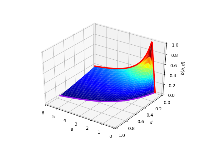
The surface in the parameters space \((\alpha,d,\beta)\). Below this surface the system has a limit cycle and above it a fixpoint.

Time evolution of the system

We can analyze the system for particular choice of parameters. There are two important examples:

Solutions which tend to the limit cycle:

If once chooses the parameters \(\alpha = 1,\; \beta =t 0.1,\; d = 0.1 0\) then the system has a unstable fix point inside the first quadrant, at \(x_0=y_0=\newcommand{\Bold}[1]{\mathbf{#1}}\frac{1}{20} \, \sqrt{41} - \frac{1}{20}\). Both eigenvalues of Jacobian in this posit have positive real parts, thus the point is unstable. On the other hand the inspection of the vector field indicates that the flow in the phase space is transporting into the \((0,1)\times(0,1)\) region. It suggests that the system can have at least limit cycle.

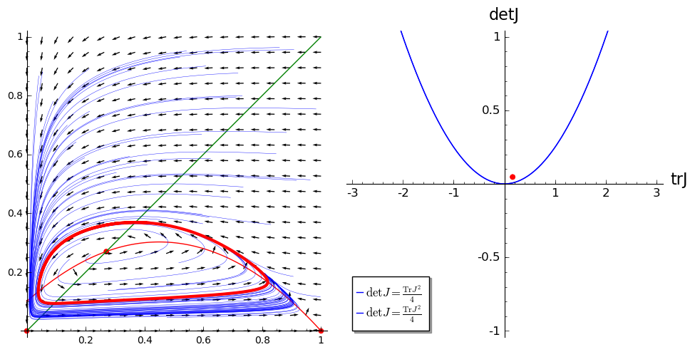
The phase portrait of a system and the location of the \(\mathrm{Tr}J\) and \(\det J\) respective to critical curve.

Alternatively, one can figure out the stablity of the fix point from the sign of trace and determinant of the Jacobian in that point.

Experiment with Sage!

Check the sign of trace and determinant of the Jacobian of the fix point for parameters \(\alpha = 1,\; \beta =t 0.1,\; d= 0.1\). Calculate eigenvalues and compare if the same conclusions on the stablility of the fix point can be drawn. Use:

• J.trace()

• J.det()

• J.eigenvalues()

Experiment with Sage!

Draw time solution to the system for parameters point \(\alpha = 1,\; \beta =0.1,\; d= 0.1\).

Solutions which tend to the stable spiral

If once chooses the parameters \(\alpha = 1,\; \beta =t 0.1,\; d = 1.\) then the system has a unstable fix point inside the first quadrant, at \(x_0=y_0=\newcommand{\Bold}[1]{\mathbf{#1}}\frac{1}{20} \, \sqrt{41} - \frac{1}{20}\). Both eigenvalues of Jacobian in this posit have positive real parts, thus the point is unstable. On the other hand the inspection of the vector field indicates that the flow in the phase space is transporting into the \((0,1)\times(0,1)\) region. It suggests that the system can have at least limit cycle.

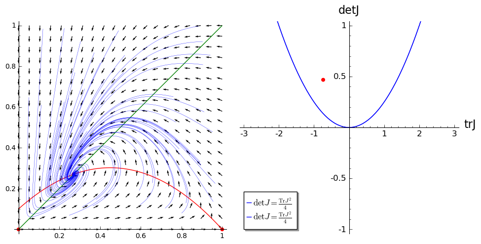
The phase portrait of a system and the location of the \(\mathrm{Tr}J\) and \(\det J\) respective to critical curve.

Experiment with Sage!

Draw time solution to the system for parameters point \(\alpha = 1,\; \beta =0.1,\; d= 1\).