Analysis of the May model with SAGE
Dimensionless the May model reads:
where we have defined the following dimensionless parameters:
This scaling procedure leads to a set of two differential equations with only three parameters. The dimensionless time is scaled to the reproducinng rate \(r\) of prey. The parameter \(\beta\) is the relation of the reproducing rate of predators \(s\) to the reproducing rate of prey \(r\). If \(\beta \lt 1\) then the reproducting tempo of predators is smaller than prey and therefore the prey population can survive. On the other hand, f \(\beta \gt 1\) then the reproducting tempo of predators is greater than for prey and therefore the prey population can become extinct (can fail to survive). But because the set of two equations is nonlinear, such simplified considerations cannot be fully true. We have to use precise mathematical methods to check this.
STATIONARY STATES
Stationary states are determined by a set of two algebraic equations:
One stationary state can easily be found:
In theis state there are no predators and the state of prey is the same as in the Verhulst system. We should cjeck whether this stse is stable.
From the second equation we find that \(y=x\) solves this equation. We put it in the first equation and then the other stationary states are determined by the equations:
From the second equation we obtain the condition:
It is a trinomial square and we take into account only non-negative solutions of this equation, \(x \ge 0\). Discriminant is always positive, namely,
So, the second stationary state is
Let us note that this state does not depend on the parameter \(\beta\), i.e. on the birth rate of prey and predators.
STABILITY OF STATIONARY STATES
In the first step, we calculate the Jacobi matrix:
In the second step, we determine the eigenvalues of the Jacobi matrix \(|J -\lambda I|=0\):
For the stationary state \((1, 0)\) one gets:
and the eigenvalues are: \(\lambda_{1} = -1, \quad \lambda_{2} = \beta > 0\). So, this state is not stable because one eigenvalue is positive, \(\lambda_{2} \gt 0\). A small perturbation will displace the system from this state.
For the second stationary state the problem of stability is more complicated because the Jacobi matrix takes the form
We used the equation for the stationary state to transform the term \(J_{11}\) to the form as in this matrix. One can try to determine the eigenvalues of this matrix. But it is not good way. What we want to know is the sign of a real part (positive or negative) of both eigenvalues \((\lambda_1, \lambda_2)\). Because this matrix is \(2 \times 2\), we get a trinomial square for \(\lambda\). The conditions for its negative part reads:
- WORK:
Show that for arbitrary (positive) values of parameters \(\alpha, \beta, d\), the second condition \(\mbox{det} \,J \gt 0\) is always fulfiled.
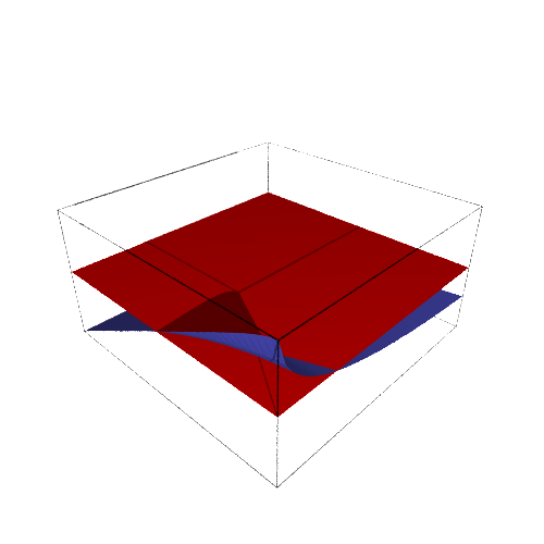
The first condition for the stability of the state \((x_2, y_2)\) takes the form:
Because \(x_2\) depends on 2 parameters \(\alpha\) and \(d\), the right-hand side defines the surface in the 3-dimensional space.
[50]:
var('a b d x y')
ode_lotka=[x*(1-x)-(a*x*y)/(x+d),b*y*(1-y/x)]
show(ode_lotka)
[51]:
J = jacobian(ode_lotka,[x,y])
[52]:
detJ = det(J)
[53]:
detJ.variables()
[53]:
(a, b, d, x, y)
[54]:
detJ.subs({a:1})
[54]:
(b*(y/x - 1) + b*y/x)*(2*x + y/(d + x) - x*y/(d + x)^2 - 1) + b*y^2/((d + x)*x)
[55]:
for sol_ in solve(ode_lotka,[x,y]):
    show(sol_)
[56]:
sols = solve(ode_lotka,[x,y])
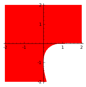
We check if solutions are in first quadrant of coordinate system. We need it for positive \(a\) and \(d\).
[57]:
sol_ = sols[4]
region_plot(sol_[0].rhs()>=0 and sol_[1].rhs()>=0,(a,-2,2),(d,-2,2),incol='red',plot_points=400,figsize=4)
/usr/local/lib/SageMath82/local/lib/python2.7/site-packages/sage/plot/contour_plot.py:1515: RuntimeWarning: invalid value encountered in less
  neg_indices = (xy_data_arrays < 0).all(axis=0)
[57]:
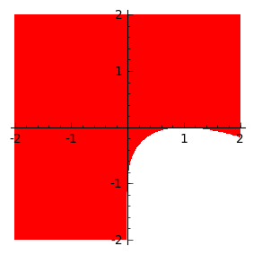
We check if \(\det J\) is positive al all parametres. If \(b>0\) then \(\frac{\det J}{b}\) depends only on \((a,d)\):
[58]:
(detJ.subs(sol_)/b).full_simplify().variables()
[58]:
(a, d)
thus we can check numerically using region plot if it takes positive values for all \((a,d)\) in the first quadrant of parameter space.
[59]:
region_plot((detJ.subs(sol_)/b).full_simplify()>0,(a,-2,2),(d,-2,2),incol='red',figsize=4,plot_points=400)
[59]:
[60]:
trJ = J.trace()
One can solve equation \(tr J==0\) for \(b\) and the inequality becomes: \(b< \mbox{trJ_b}\).
[61]:
trJ_b = trJ.subs(sol_).solve(b)[0].rhs()
[62]:
trJ_b.variables()
[62]:
(a, d)
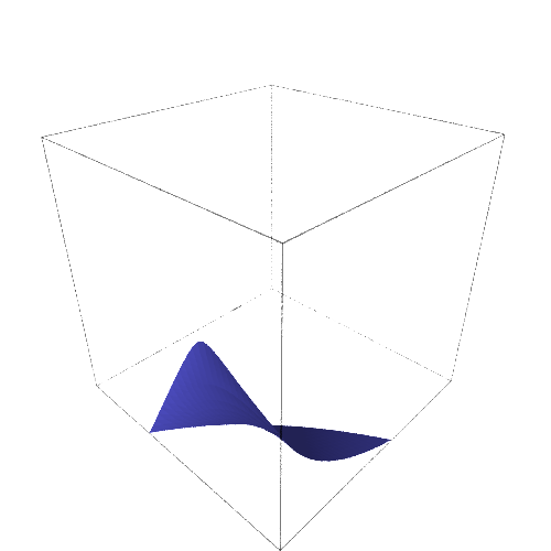
[63]:
implicit_plot3d(trJ.subs(sol_),(a,1e-3,1.41),(d,1e-3,.61),(b,0,1.5)).show(viewer='tachyon')
[64]:
plt = plot3d(trJ_b,(a,1e-3,1),(d,1e-3,1))
plt += plot3d(0,(a,0,1),(d,0,1),color='red')
plt.show(viewer='tachyon')
[65]:
implicit_plot(trJ_b,(a,0,2),(d,0,1))
[65]:
[69]:
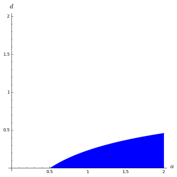
plt_cond_trJ = region_plot( trJ_b>0,(a,0,2),(d,+1e-4,2),plot_points=400,
                          axes_labels=[r'$a$',r'$d$'])
plt_cond_trJ
[69]:
[79]:
var('X')
expr = trJ_b.subs((a^2 + 2*a*d + d^2 - 2*a + 2*d + 1) == X)
expr.full_simplify()
[79]:
1/2*(4*a^3 + 2*(a - 1)*d^2 - 10*a^2 + 2*(3*a^2 + a - 2)*d - (3*a^2 - d^2 + X - 4*a + 1)*sqrt(X) + 8*a - 2)/(a^2 + d^2 - sqrt(X)*(a - d - 1) - 2*a + 2*d + 1)
[80]:
expr.subs([sqrt(X)])
[80]:
1/2*(4*a^3 + (2*a + sqrt(X) - 2)*d^2 - a^2*(3*sqrt(X) + 10) + 2*(3*a^2 + a - 2)*d + 4*a*(sqrt(X) + 2) - X^(3/2) - sqrt(X) - 2)/(a^2 + d^2 - a*(sqrt(X) + 2) + d*(sqrt(X) + 2) + sqrt(X) + 1)
[57]:
var('a,d,b,x,y,t')
ode_lotka=vector([x*(1-x)-(a*x*y)/(x+d),b*y*(1-y/x)]);
[58]:
b_in = 0.12
d_in = 0.15
a_in = 1.2
p = {a:a_in, d:d_in, b:b_in}
[317]:
b_in<trJ_b.subs(p).n()
[317]:
True
[49]:
plt_cond_trJ + point( (a_in,d_in),color='red',size=30,zorder=10,plot_points=400)
---------------------------------------------------------------------------
NameError                                 Traceback (most recent call last)
<ipython-input-49-00ec68891fc8> in <module>()
----> 1 plt_cond_trJ + point( (a_in,d_in),color='red',size=Integer(30),zorder=Integer(10),plot_points=Integer(400))

NameError: name 'plt_cond_trJ' is not defined
[319]:
ode_lotka.subs(p).list()
[319]:
[-(x - 1)*x - 1.20000000000000*x*y/(x + 0.150000000000000),
 -0.120000000000000*y*(y/x - 1)]
[3]:
ode_lotka
[3]:
(-(x - 1)*x - a*x*y/(d + x), -b*y*(y/x - 1))
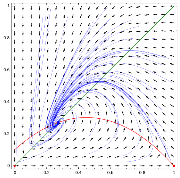
[116]:
def phase_may(p, xylims  = [(x,1e-4,1),(y,1e-4,1)]):
    pkts = solve(ode_lotka.subs(p).list(),[x,y])

    colors = ['red','green','blue']


    plt_fixpoints = point([vector([x,y]).subs(pkt) for pkt in pkts if pkt[0].rhs()>=0 and pkt[1].rhs()>=0],color='red',size=30)


    plt_null = sum([implicit_plot(eq,*xylims,color=c) for eq,c in zip(ode_lotka.subs(p),colors)])
    plt_phase = plot_vector_field(ode_lotka.subs(p).normalized(),*xylims,plot_points=20)
    plt_phase += plt_fixpoints+plt_null

    ith_1st = [i for i,pkt in enumerate(pkts) if pkt[0].rhs()>0 and pkt[1].rhs()>0 ][0]

    Jp = jacobian(ode_lotka.subs(p),[x,y]).subs(pkts[ith_1st])

    has_LC = False

    if Jp.trace()>0:
        print("fix point is unstable")
        has_LC = True

    print('detJ>trJ^2/4?',Jp.det().n()>Jp.trace().n()^2/4)

    plt_trajs=Graphics()

    ics_lst = []
    for dy in srange(0.01,0.71,0.05):
        ics_lst.append( vector((x,y+dy)).subs(pkts[ith_1st]) )

    ics_lst = [ (random(),random()) for i in range(50)]

    for ics in ics_lst:
        T = srange(0,50,0.01)
        traj = desolve_odeint(ode_lotka.subs(p),ics,T,[x,y])

        plt_trajs += line(traj,thickness=0.3)

    if has_LC:
        T = srange(0,350,0.2)
        traj_lc = desolve_odeint(ode_lotka.subs(p),(1,1.23),T,[x,y])[-205:,:]
        plt_traj_lc = line(traj_lc,color='red',zorder=11,thickness=3)


    plt_phase += plt_trajs
    if has_LC:
        plt_phase += plt_traj_lc
    return plt_phase,pkts[ith_1st],Jp.trace(),Jp.det()
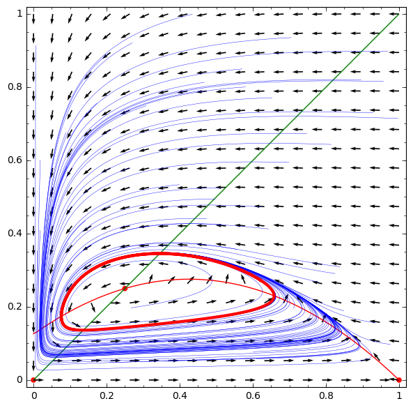
[63]:
phase_may(p)[0]
fix point is unstable
('detJ>trJ^2/4?', True)
[63]:
[178]:
@interact
def _(a_in = slider(0,2,0.01,default=1.0),\
        b_in = slider(0,2,0.01,default=0.1),\
        d_in = slider(0,2,0.01,default=0.1) ):

    p = {a:a_in,d:d_in,b:b_in}
    plt,pkt,tr,det_ = phase_may(p)
    plt_dettr = plot(x^2/4, (x,-3,3),ymin=-1,ymax=1,legend_label=r'$\detJ=\frac{\mathrm{Tr}J^2}{4}$')
    plt_dettr += point((tr,det_),color='red',size=30,axes_labels=['trJ','detJ'],legend_label="")
    #plt.show(figsize=6)
    #plt_dettr.show(figsize=5)
    graphics_array([[plt,plt_dettr]]).show(figsize=[10,5])
[ ]:
[169]:
var('a,d,b,x,y,t')
ode_lotka=vector([x*(1-x)-(a*x*y)/(x+d),b*y*(1-y/x)]);
[170]:
p = {a:1.0, d:0.1, b:1}
[171]:
sol = solve(list(ode_lotka.subs(p)),[x,y])[4]
[172]:
J = jacobian(ode_lotka.subs(p),[x,y]).subs(sol).n()
show(J)
[173]:
J.trace(),
[173]:
(-0.737484256802092,)
[174]:
J.det()
[174]:
0.467328044930449
[175]:
J.trace()^2/4
[175]:
0.135970757257733
[176]:
xylims = [(x,1e-4,1),(y,1e-4,1)]
[177]:
phase_may(p,xylims=[(x,+1e-4,1),(y,+1e-4,1)])[0]
('detJ>trJ^2/4?', True)
[177]:
[ ]:
[157]:
eps = 1e-3
solve(ode_lotka.subs(p).subs(y==eps)*vector([0,1])>=0,x)
[157]:
[[x < 0], [x >= (1/1000)]]
[143]:
solve(ode_lotka.subs(p).subs(x==0.00001)*vector([1,0])>0,x)
[143]:
[[y < (10001/100001)]]
[ ]:
[166]:
J
[166]:
[ 0.262515743197908 -0.729843788128358]
[ 0.100000000000000 -0.100000000000000]
[ ]:
[ ]:
[ ]:
[ ]:
[ ]:
[ ]:
[ ]:
[ ]:
[ ]:
[ ]:
[ ]:
[385]:
@interact
def May_phase(a_in = slider(0,2,0.01,default=1.0),\
        b_in = slider(0,2,0.01,default=0.1),\
        d_in = slider(0,2,0.01,default=0.1) ):
    p = {a:a_in,d:d_in,b:b_in}
    ode_lotka_num =[i.subs(p) for i in ode_lotka]
    pkt_osob=solve(ode_lotka_num,x,y, solution_dict=True)
    x_osobliwy,y_osobliwy=0,0
    plt_pkt=[]
    for n_pkt,pkt in enumerate(pkt_osob):
       x_osobliwy,y_osobliwy=pkt[x].n(),pkt[y].n()
       plt_pkt.append(point([x_osobliwy,y_osobliwy],size=30,color='red') )
       JJ=jacobian(ode_lotka_num,[x,y])
       JJ0=JJ.subs({x:x_osobliwy+1e-8,y:y_osobliwy+1e-8})
       print n_pkt+1,":",x_osobliwy.n(digits=3),y_osobliwy.n(digits=3),vector(JJ0.eigenvalues()).n(digits=3)
       if pkt[x]>0 and pkt[y]>0 :
           print "Czy pkt. jest stabilny?",bool(b_in>f(a_in,d_in))
           print "detJ>(TrJ/2)^2",(detJ.subs(sol_)-(trJ.subs(sol_)/2)^2).subs(p).n()
    plt1 = plot_vector_field(vector(ode_lotka_num)/vector(ode_lotka_num).norm(),(x,-0.1,2),(y,-0.1,2))
    #plt2a = implicit_plot(ode_lotka_num[0],(x,-0.10,2),(y,-0.10,2),color='green')
    plt2a = plot(solve(ode_lotka_num[0],y)[0].rhs(),(x,-0.10,2),ymin=-0.10,ymax=2, color='green')
    show(ode_lotka_num)
    plt2b = implicit_plot(ode_lotka_num[1],(x,-0.10,2),(y,-.010,2),color='blue',xmin=-0.03)
    T = srange(0,123,0.1)
    sol1 = desolve_odeint(vector(ode_lotka_num), [0.82,0.85], T, [x,y])
    plt_solution = list_plot(sol1.tolist(), plotjoined=True, color='brown')
    show( sum(plt_pkt)+plt1+plt2a+plt2b+plt_solution )
[93]:
var('Delta',latex_name='\sqrt{\Delta}')
subDelta = sqrt(a^2 + 2*(a + 1)*d + d^2 - 2*a + 1)==Delta
[94]:
sol_[1].rhs().subs(subDelta)
[94]:
1/2*Delta - 1/2*a - 1/2*d + 1/2
[95]:
detJ.subs(sol_).subs(subDelta).expand().full_simplify()
[95]:
-((Delta + 2*a + 2)*b*d^2 + b*d^3 - (Delta^2 - a^2 + 2*a - 1)*b*d - (Delta^3 + Delta*a^2 + 2*Delta^2 - 2*(Delta^2 + Delta)*a + Delta)*b)/(Delta^2 - 2*(Delta + 1)*a + a^2 + 2*(Delta - a + 1)*d + d^2 + 2*Delta + 1)
[96]:
point1 = sols[0]
point2 = sols[1]
point3 = sols[4]
#point3 = map(lambda x:x.subs(subDelta),point3)
[97]:
point3
[97]:
[x == -1/2*a - 1/2*d + 1/2*sqrt(a^2 + 2*(a + 1)*d + d^2 - 2*a + 1) + 1/2,
 y == -1/2*a - 1/2*d + 1/2*sqrt(a^2 + 2*(a + 1)*d + d^2 - 2*a + 1) + 1/2]
[364]:
trJ.subs(point3).simplify().numerator()
[364]:
a^3 - a^2*b + a^2*d + 2*a*b*d + a*d^2 - b*d^2 + d^3 - 3*sqrt(a^2 + 2*a*d + d^2 - 2*a + 2*d + 1)*a^2 + 2*sqrt(a^2 + 2*a*d + d^2 - 2*a + 2*d + 1)*a*b - 2*sqrt(a^2 + 2*a*d + d^2 - 2*a + 2*d + 1)*b*d + sqrt(a^2 + 2*a*d + d^2 - 2*a + 2*d + 1)*d^2 + 3*(a^2 + 2*a*d + d^2 - 2*a + 2*d + 1)*a - 4*a^2 - (a^2 + 2*a*d + d^2 - 2*a + 2*d + 1)*b + 2*a*b - (a^2 + 2*a*d + d^2 - 2*a + 2*d + 1)*d - 6*a*d - 2*b*d - (a^2 + 2*a*d + d^2 - 2*a + 2*d + 1)^(3/2) + 4*sqrt(a^2 + 2*a*d + d^2 - 2*a + 2*d + 1)*a - 2*sqrt(a^2 + 2*a*d + d^2 - 2*a + 2*d + 1)*b + 5*a - b - 3*d - sqrt(a^2 + 2*a*d + d^2 - 2*a + 2*d + 1) - 2
[365]:
detJ.subs(point3).simplify().numerator().show()
2d

[98]:
(detJ.subs(sol_)-(trJ.subs(sol_)/2)^2).subs({a:1,d:1,b:.1}).n()
[98]:
0.00357530887414820
[ ]:
[99]:
point3
[99]:
[x == -1/2*a - 1/2*d + 1/2*sqrt(a^2 + 2*(a + 1)*d + d^2 - 2*a + 1) + 1/2,
 y == -1/2*a - 1/2*d + 1/2*sqrt(a^2 + 2*(a + 1)*d + d^2 - 2*a + 1) + 1/2]
[100]:
var('x0')
[100]:
x0
[104]:
trJ.subs({x:x0,y:x0}).factor().numerator().collect(b).show()
[ ]:
[366]:
y_z_pierwszego=solve(ode_lotka[0],y,solution_dict=True)[0]
drugie=ode_lotka[1].subs(y_z_pierwszego)
show(drugie)
show(solve(drugie,x,solution_dict=True)[0])
x_0=x.subs(solve(drugie,x,solution_dict=True)[1])
y_0=y_z_pierwszego[y].subs({x:x_0}).expand()
show(x_0)
show( y_0 )
[ ]:
[367]:
ode_lotka[0].diff(x).show()
[368]:
JJ = jacobian(ode_lotka,[x,y])
show(JJ)
[370]:
#mamy x0=y0 ;-)
var('x0')
JJ0 = JJ.subs({x:x0,y:x0})
[371]:
show(JJ0)
[372]:
show(JJ0.trace())
[398]:
trJ.subs({x:x0,y:x0}).operands()
[398]:
[-b, -a*x0/(d + x0), -2*x0, a*x0^2/(d + x0)^2, 1]
[395]:
expr_murray = x0*(a*x0/(x0-d)^2-1)
expr_murray.show()
[405]:
show( JJ0.trace().subs({x0:x_0})+b )
[19]:
p={a:1.23,d:1.01}
show( JJ0.trace().subs({x0:x_0}).subs(p) )
expr_murray.subs({x0:x_0}).subs(p)
[19]:
1.35696399470668
[598]:
var('a,d,b,x,y,t')
ode_lotka=[x*(1-x)-(a*x*y)/(x+d),b*y*(1-y/x)];
#Murray eq. 3.28
f(a,d)=(a-sqrt(  (1-a-d)^2+4*d) )*(1+a+d-sqrt((1-a-d)^2+4*d))/(2*a)
@interact
def myf(a_in = slider(0,2,0.01,default=1.0),b_in = slider(0,2,0.01,default=0.1),d_in = slider(0,2,0.01,default=0.1) ):
    p={a:a_in,d:d_in,b:b_in}
    ode_lotka_num=[i.subs(p) for i in ode_lotka]
    pkt_osob=solve(ode_lotka_num,x,y, solution_dict=True)
    x_osobliwy,y_osobliwy=0,0
    plt_pkt=[]
    for n_pkt,pkt in enumerate(pkt_osob):
       x_osobliwy,y_osobliwy=pkt[x].n(),pkt[y].n()
       plt_pkt.append(point([x_osobliwy,y_osobliwy],size=30,color='red') )
       JJ=jacobian(ode_lotka_num,[x,y])
       JJ0=JJ.subs({x:x_osobliwy+1e-8,y:y_osobliwy+1e-8})
       print n_pkt+1,":",x_osobliwy.n(digits=3),y_osobliwy.n(digits=3),vector(JJ0.eigenvalues()).n(digits=3)
       if pkt[x]>0 and pkt[y]>0 :
           print "Czy pkt. jest stabilny?",bool(b_in>f(a_in,d_in))
           print "detJ>(TrJ/2)^2",(detJ.subs(sol_)-(trJ.subs(sol_)/2)^2).subs(p).n()
    plt1 = plot_vector_field(vector(ode_lotka_num)/vector(ode_lotka_num).norm(),(x,-0.1,2),(y,-0.1,2))
    #plt2a = implicit_plot(ode_lotka_num[0],(x,-0.10,2),(y,-0.10,2),color='green')
    plt2a = plot(solve(ode_lotka_num[0],y)[0].rhs(),(x,-0.10,2),ymin=-0.10,ymax=2, color='green')
    show(ode_lotka_num)
    plt2b = implicit_plot(ode_lotka_num[1],(x,-0.10,2),(y,-.010,2),color='blue',xmin=-0.03)
    T = srange(0,123,0.1)
    sol1 = desolve_odeint(vector(ode_lotka_num), [0.82,0.85], T, [x,y])
    plt_solution = list_plot(sol1.tolist(), plotjoined=True, color='brown')
    show( sum(plt_pkt)+plt1+plt2a+plt2b+plt_solution )
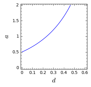
[18]:
var('a,d',domain='real')
f(a,d)=(a-sqrt(  (1-a-d)^2+4*d) )*(1+a+d-sqrt((1-a-d)^2+4*d))/(2*a)
show(f)
plt2 = implicit_plot( f(a,d),(d,0,.61),(a,0,2),aspect_ratio=0.3,  figsize=(6, 3), axes_labels=[r'$d$','$a$'] )
plt2
[18]:
[457]:
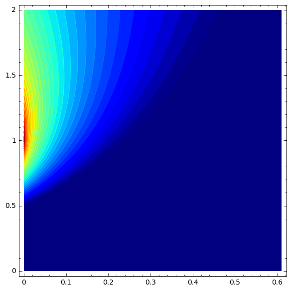
b_ad = (trJ.subs(point3)).solve(b)[0].rhs().full_simplify()
[458]:
b_ad.full_simplify()
[458]:
(2*a^3 + (a - 1)*d^2 - 5*a^2 + (3*a^2 + a - 2)*d - (2*a^2 + (a + 1)*d - 3*a + 1)*sqrt(a^2 + 2*(a + 1)*d + d^2 - 2*a + 1) + 4*a - 1)/(a^2 + d^2 - sqrt(a^2 + 2*(a + 1)*d + d^2 - 2*a + 1)*(a - d - 1) - 2*a + 2*d + 1)
[500]:
contour_plot(b_ad,(d,1e-4,.61),(a,0,2),aspect_ratio=.31,contours=srange(0,1.1,0.031),cmap='jet',plot_points=432)
[500]:
[501]:
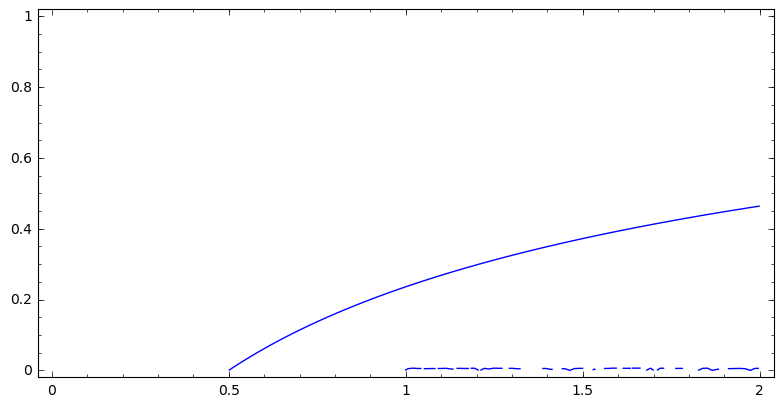
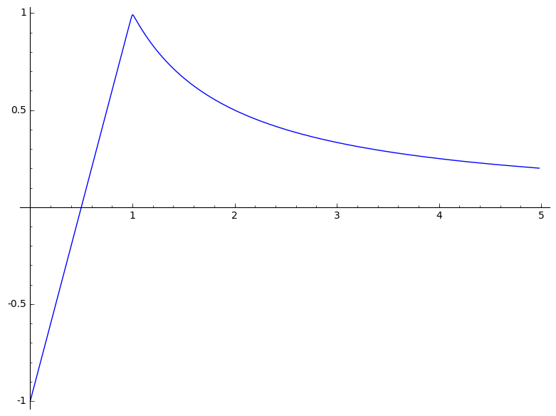
b_ad.subs(d==1e-4).show()
[507]:
plot(b_ad.subs(d==1e-5),(a,0.0,4.98))
[507]:
[ ]:
[ ]:
Pod tą płaszczyzną
mamy cykl graniczny:
[20]:
var('a,d')
f(a,d)=(a-sqrt(  (1-a-d)^2+4*d) )*(1+a+d-sqrt((1-a-d)^2+4*d))/(2*a)
show(f)
sol1=solve(f(a,d)==0, d)
show(sol1)
dm_expr=sol1[1].rhs()
assume(a>0)
f(a,0).full_simplify()
[20]:
1/2*(2*a^2 - a*(2*abs(a - 1) + 1) - abs(a - 1) + 1)/a
[31]:
forget()
assume(a<1)
f(a,0).simplify()
[31]:
1/2*(a - sqrt((a - 1)^2) + 1)*(a - sqrt((a - 1)^2))/a
[53]:
def b2(a,d):
    return (a-np.sqrt(  (1-a-d)**2+4*d) )*(1+a+d-np.sqrt((1-a-d)**2+4*d))/(2*a)
def dm(a):
    return -a + np.sqrt(a**2 + 4*a) - 1
def bm(a):

    if type(a) == np.ndarray:
        out = np.empty_like(a)
        a_lt_1 = a[a<1]
        a_gt_1 = a[a>=1]
        out[a<1] = 1/a_lt_1

        out[a>=1] =  0.5*(a_gt_1 - np.sqrt((a_gt_1 - 1)**2) + 1)*(a_gt_1 - np.sqrt((a_gt_1 - 1)**2))/a_gt_1
        return out
    else:
        if a>1:
            return 1/a
        else:
            return 0.5*(a - np.sqrt((a - 1)**2) + 1)*(a - np.sqrt((a - 1)**2))/a


from mpl_toolkits.mplot3d import Axes3D
import matplotlib
from matplotlib import cm
from matplotlib import pyplot as plt
step = 0.04
maxval = 1.0
fig = plt.figure()
ax = fig.add_subplot(111, projection='3d',azim=134)
x = np.linspace(0.5,6,115)
y = np.linspace(0.00,1.,35)
X,Y = np.meshgrid(x,y)
# transform them to cartesian system
X,Y = X,Y*(np.sqrt(X**2+4*X)-(1.0+X))
#Y[:,i((X[7,0]**2+4*X[7,0])**0.5 - (1+X[7,0]) )
#0.99*d(:,i)*((a1.^2+4.*a1)^0.5 - (1+a1) )
Z = b2(X,Y)
ax.plot_surface(X, Y, Z, rstride=2, cstride=2, cmap=cm.jet)
#ax.plot_surface(X, Y, Z,  cmap=cm.jet)
#ax.plot_wireframe(X, Y, Z)
ax.set_zlim3d(0, 1)
ax.set_xlim3d(0, 3)
ax.set_ylim3d(0, .7)
ax.set_xlabel(r'$a$')
ax.set_ylabel(r'$d$')
ax.set_zlabel(r'$b(a,d)$')
ax.plot(x, dm(x), np.zeros_like(x), color=(.6,.1,.92),linewidth=3)
ax.plot(x,np.zeros_like(x), bm(x),  color='red',linewidth=3)
ax.plot([0],[0],[0])
ax.view_init(elev=35, azim=134)
plt.show()#plt.savefig("1.png")
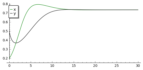
Rozwiązania dążące do stabilnego stanu stacjonarnego: \(a \in (0, 0.5), \beta \gt 0, d \gt 0\)
[28]:
var('x,y')
a, b, d = 0.3, 0.35, 0.1
T = srange(0,30,0.01)
sol2 = desolve_odeint(\
 vector([x*(1-x) - (a*x*y/(x+d)), b*y*(1-y/x)]),\
 [0.2, 0.5],T,[x,y])
line( zip ( T,sol2[:,0]) ,color='green', figsize=(6, 3), legend_label="x")+\
 line( zip ( T,sol2[:,1]) ,color='black',legend_label="y")
[28]:
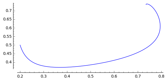
[30]:
a, b, d = 0.3, 0.35, 0.1
F(x,y)=x*(1-x) - a*x*y/(x+d)
G(x,y)= b*y*(1-y/x)
T = srange(0,30,0.01)
sol1=desolve_odeint(vector([F,G]), [0.2,0.5], T, [x,y])
list_plot(sol1.tolist(), plotjoined=True,  figsize=(6, 3))
[30]:
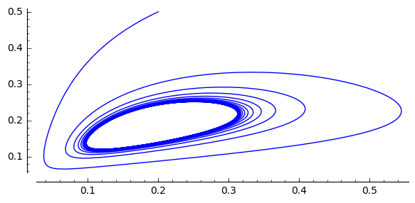
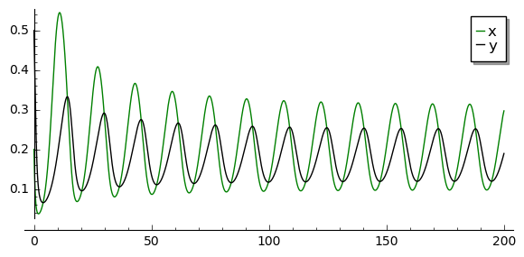
Rozwiązania dążące do stabilnego cyklu granicznego: \(a \gt 0.5 , \beta \gt 0, d \gt 0\)
[31]:
var('x,y')
a, b, d = 1.3, 0.33, 0.1
T = srange(0,200,0.01)
sol2=desolve_odeint(\
 vector([x*(1-x) - (a*x*y/(x+d)), b*y*(1-y/x)]),\
 [0.2, 0.5],T,[x,y])
line( zip ( T,sol2[:,0]) ,color='green', figsize=(6, 3), legend_label="x")+\
 line( zip ( T,sol2[:,1]) ,color='black',legend_label="y")
[31]:
[33]:
a, b, d = 1.3, 0.33, 0.1
F(x,y)=x*(1-x) - a*x*y/(x+d)
G(x,y)= b*y*(1-y/x)
T = srange(0,250,0.01)
sol1=desolve_odeint(vector([F,G]), [0.2,0.5], T, [x,y])
list_plot(sol1.tolist(), plotjoined=True,  figsize=(6, 3))
[33]: