Ludwig et al. Model for Tumor Growth

This is a one dimensional model applied to description of ecological systems, in particular the spruce budworm-forest interaction in the eastern North America (D. Ludwig, D. D. Jones and C. S. Holling, “Qualitative Analysis of Insect Outbreak Systems: The Spruce Budworm and Forest”, The Journal of Animal Ecology, Vol. 47, p. 315, 1978). Introduction of this model is presented in the previous section. This model is an example which can be applied to variety of phenomena. The interesting example is modeling of tumor growth with immunization. In the absence of an immune reaction, tumor evolution is thought to follow a limited growth law that can be described by e.g. the Verhulst mechanism. The carrying capacity measures the greatest possible number to which the tumor cells can be extended. The carrying capacity is determined by the resources of the system in which the tumor will be embedded. The influence of the immune system on tumor growth is represented by the predation term in the Ludwig model. The immune system try to eradicate the tumor cells and acts as predator in the population dynamics: The lymphocytes migrate to the tumor site, recognize the tumor cells, and initiate a powerful immune reaction that ends up in the destruction of the tumor tissue. Whenever not all of the tumor cells are destroyed during the elimination phase, a transition into the equilibrium phase will occur. The effector cells of the immune system further attack the tumor and exert a selective pressure on the cancer cells. In this manner only the susceptible cancer cell variants will be eliminated by the immune system, whereas tumor cell clones that are nonimmunogenic will survive leading to a sculpting of the immunogenic phenotype of the tumor. We recall an evolution equation introduced for the first time in the Ludwig et al. paper. It has the form:

\[\frac{dN}{dt} = R N \left( 1-\frac{N}{K}\right) - \frac {BN^2}{A^2+N^2} = a(N) - b(N),\qquad (1)\]

The first term is the Verhulst one which describes the growth process of tumor cells. The second term describes the influence of the immune system which acts as a predator: it destroys the tumor cells. Both terms have similar interpretation as for the budworm population dynamics. It is the first example of the model which exhibits bifurcation phenomena. In this sense, it is non-trivial. It is not clinically relevant model but should be considered as an idealization and the first step to construct more realistic models which, in the future, could be able to forecast clinical outputs, such as overall response to treatment and time to progression, which will provide opportunities for guided intervention and improved patient care.

We should rescale this equation to the dimensionless form and reduce a number of parameter. We define ne values as:

\[x=N/A, \quad r= RA/B, \quad k=K/A, \quad \tau = (B/A) t . \qquad (2)\]

In these new variables the Ludwig equation reads:

\[\frac{dx}{d\tau} = r x ( 1-\frac{x}{k}) - \frac {x^2}{1+x^2} = f(x) = - \frac{dU(x)}{dx}, \qquad (3)\]

Here we introduced the “potential” \(U(x)\) defined by the derivative of the “force” \(f(x)\). It can be obtained by integration of the function \(-f(x)\). Note that the scaling reduces a number of paramters from 4 to 2: \(r\) and \(k\) which have the same interpretation as in the Verhulst model.

EXCERCISE: Rescale this equation in the same way as for the Verhulst model. Introduce the new variables \(y=N/K\) and \(s=r t\). This scaling is not as convenient as the first scaling. Why?

Below we show both the function \(f(x)\) and the potential \(U(x)\) for some fixed values of parameters.

var('r k x y',domain='real')
f(x)=r*x*(1-x/k) - x^2/(1+x^2)
show(f)
U=-f.integrate(x)
show(U)

$$\newcommand{\Bold}[1]{\mathbf{#1}}x \ {\mapsto}\ -r x {\left(\frac{x}{k} - 1\right)} - \frac{x^{2}}{x^{2} + 1}$$ $$\newcommand{\Bold}[1]{\mathbf{#1}}x \ {\mapsto}\ -\frac{{\left(3 \, k x^{2} - 2 \, x^{3}\right)} r}{6 \, k} + x - \arctan\left(x\right)$$

In the above cell, the first expression is the function \(f(x)\). Note that it is rewritten by Sage in a different way than originally as in the equation (3). The second line is calculation of the potential \(U(x)\).

Stationary states

The stationary states \(x_s\) are determined by roots of the equation \(f(x)=0\). Below the above function \(f(x)\) is depicted for fixed values of the parameters \(r\) and \(k\). One can notice that for this set of parameters there are 4 roots, i.e. 4 stationary states \(x_s = 0, x_1, x_2, x_3\).

plot( f(x).subs({r:.4,k:14}),(x,0,13),figsize=(7,2),axes_labels=[r'$x$',r'$f(x)$'],tick_formatter='latex')

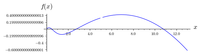
• :math:`r=0.4, qquad k=14`

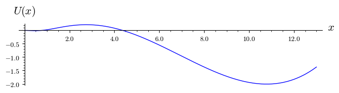
plot( U(x).subs({r:.4,k:14}),(x,0,13),figsize=(7,2),axes_labels=[r'$x$',r'$U(x)$'],tick_formatter='latex')

plot( U(x).subs({r:.4,k:14}),(x,-0.2,1),figsize=(7,2),axes_labels=[r'$x$',r'$U(x)$'])

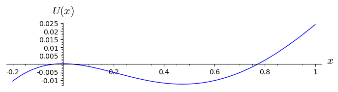
The corresponding potential \(U(x)\) possesses 4 extrema: 2 maxima and 2 minima. We enlarged the second figure for the potential to show its maximum for \(x=0\) and the minimum in the vicinity \(x=0.47\). So, \(x_s=0\) is unstable and \(x_s \approx 0.47\) is stable.

Graphical solution

The equation determining stationary states \(f(x)=0\) can be rewritten in an equivalent form as:

\[r x ( 1-\frac{x}{k}) = \frac {x^2}{1+x^2}\]

This form allows to find stationary solutions in a graphical way. One of the stationary state is \(x=0\). Other states are find by the solution of the equation

\[r ( 1-\frac{x}{k}) = \frac {x}{1+x^2}\]

It can be solved graphically. The function in the right hand side has no parameters and can be plotted. The function in the left hand side is a straight line with two parameters. They can be changed. It is done below. You can change the parameters \(k\) and \(r\) using sliders and observe the intersections of both functions which determine the stationary states.

NOTE: the straight line intersects the axis OX at the point \(x=k\) and intersects the axis OY at the point \(y=r\).

From the above slider it follows that the system can have non-zero stationary states. Their number may be : 1, 2 or 3. Of course, there is still \(x_s =0\). By chaging parameters, the number of stationary states can be changed. It is what is called a bifurcation phenomenon which in physics is known as phase transition. Below, a similar slider for the potential \(U(x)\) is constructed. Minima of this potential correspond to the stable stationary solutions and maxima of \(U(x)\) corresponds to unstable stationary states.

For the set of parameters \(k=12\) and \(r=0.4\), the potential \(U(x)\) has two minima and one maximum.

Below we show how to get numerically all roots of the equation \(f(x)=0\) by changing \(n\) in sol\(2[n]\) .

solutions  = solve( 0.4*x*(1-x/12) - x^2/(1+x^2),x,solution_dict=True)
show(solutions)

$$\newcommand{\Bold}[1]{\mathbf{#1}}\left[\left\{x : -\frac{1}{2} \, \sqrt{65} + \frac{9}{2}\right\}, \left\{x : \frac{1}{2} \, \sqrt{65} + \frac{9}{2}\right\}, \left\{x : 3\right\}, \left\{x : 0\right\}\right]$$

x.subs(solutions[0]).n()

0.468871125850725

x.subs(solutions[1]).n()

8.53112887414927

x.subs(solutions[2]).n()

3.00000000000000

x.subs(solutions[3]).n()

0.000000000000000

We observe that stationary states are: 0 is always unstable (maximum of the potential), 0.46887 is stable (minimum), 3 is unstable (maximum) and 8.53 is stable (minimum). It is rule that the sequence of states is -unstable-stable-unstable-stable-

Below: An analytical solution of \(f(x)=0\) obtained by the computer algebra. It is useful?

var('k r')
sols = solve( r*x*(1-x/k) - x^2/(1+x^2),x,solution_dict=True)
show( x.subs(sols[2]))

$$\newcommand{\Bold}[1]{\mathbf{#1}}\frac{2 \, \left(\frac{1}{2}\right)^{\frac{2}{3}} {\left(k^{2} - \frac{3 \, {\left(k + r\right)}}{r}\right)}}{3 \, {\left(2 \, k^{3} + 27 \, k - \frac{9 \, {\left(k + r\right)} k}{r} + \frac{9 \, \sqrt{\frac{1}{3}} \sqrt{\frac{4 \, {\left(k^{4} + 2 \, k^{2} + 1\right)} r^{3} + 4 \, k^{3} - 4 \, {\left(5 \, k^{3} - 3 \, k\right)} r^{2} - {\left(k^{4} - 12 \, k^{2}\right)} r}{r}}}{r}\right)}^{\frac{1}{3}}} + \frac{1}{3} \, k + \frac{1}{3} \, \left(\frac{1}{2}\right)^{\frac{1}{3}} {\left(2 \, k^{3} + 27 \, k - \frac{9 \, {\left(k + r\right)} k}{r} + \frac{9 \, \sqrt{\frac{1}{3}} \sqrt{\frac{4 \, {\left(k^{4} + 2 \, k^{2} + 1\right)} r^{3} + 4 \, k^{3} - 4 \, {\left(5 \, k^{3} - 3 \, k\right)} r^{2} - {\left(k^{4} - 12 \, k^{2}\right)} r}{r}}}{r}\right)}^{\frac{1}{3}}$$

Bifurcation diagram

From the graphical method of solution of \(f(x)=0\) we see that the number of stationary states depends on values of parameters \(k\) and \(r\). Assume that e.g. \(r=0.45\). One can observe that if \(k\) is small (e.g. \(k=6\)) then there is only one root of \(f(x)=0\). If \(k\) increases then the second root occurs (which is double). The further growth of \(k\) lead to the creation of the third root. A similar phenomenon can be detected when \(r\) is varied. The value of the parameter when the second root occurs is sometimes called critical. It corresponds to the double root. From this double root, two roots are created when the parameter is a little bit varied. If the function \(f(x)\) has a double root \(x_d\) then it means that it can be presented in the form:

\[f(x) = (x-x_d)^2 g(x)\]

We see that \(f(x_d)=0\) and one can check that also the derivative \(f'(x_d)=0\). It is an important property of double roots. It means that if we want to find all values of parameters for which \(f(x)\) has double roots, we have to solve a set of two equations:

\[f(x)=0 \qquad \mbox{and} \qquad f'(x)=0\]

We can devide and colore the plane of parameters \((k, r)\) for which there is one stationary state and three stationary states. The border between these two areas forms a curve which is named the bifurcation diagram.

It is presented below.

ff1=fast_callable(  x.subs(sols[0]) , vars=[r,k], domain=CDF)
ff2=fast_callable(  x.subs(sols[1]) , vars=[r,k], domain=CDF)
ff3=fast_callable(  x.subs(sols[2]) , vars=[r,k], domain=CDF)
ff4=fast_callable(  x.subs(sols[3]) , vars=[r,k], domain=CDF)
def get_n_roots(r,k):
    x0=[]
    for ff in [ff1,ff2,ff3,ff4]:
        val=ff(r,k)
        if abs(imag(val))<1e-10:
            x0.append(real(val))
    return len(x0),x0

get_n_roots(1,1)

(2, [0.5698402909980531, 0.0])

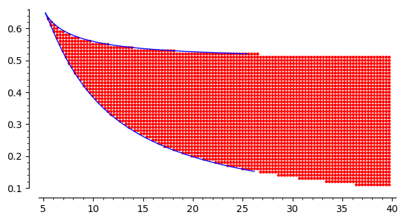
four=[]
for r_ in srange(0.01,0.9,0.01):
    for k_ in srange(1,40,.3):
      if get_n_roots(r_,k_)[0]==4:
          four.append((k_,r_))
points4=point( four ,color='red',figsize=6)
show(points4)

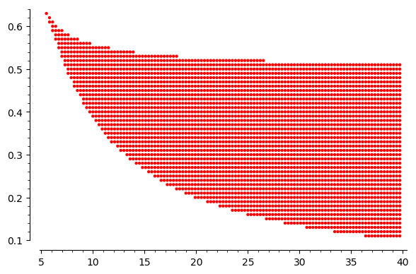
It is a result of scan of parameters to find read area where there are three stationary states. In the white part of this plane, there is one stable stationary states. The border between them is limited by the curve which can be obtained by the solution of a set of two equations: \(f(x)=0\) and \(f'(x)=0\). One can derive an analytical form for this curve from the set of two equations. It is given in a parametric form: \(\{r=F(x), k=G(x)\}\), where

\[F(x)=\frac{2x^3}{(x^2+1)^2}, \qquad G(x) = \frac{2x^3}{x^2-1} \qquad \mbox{for} \qquad x>1\]

The coordinate of the cusp can be obtained as an extremal point, i.e. from the derivative \(F'(x)=0\) or/and \(G'(x)=0\). It gives the result \(x_c=\sqrt{3}\). If we insert it to \(F\) and \(G\) then the coordinate of the casp are \((r_c \approx 0.6495, k_c\approx 5.196)\).

show(f(x))

$$\newcommand{\Bold}[1]{\mathbf{#1}}-r x {\left(\frac{x}{k} - 1\right)} - \frac{x^{2}}{x^{2} + 1}$$

expr = expand( (f(x)/x)*(x^2+1) ).full_simplify()

show(expr)

$$\newcommand{\Bold}[1]{\mathbf{#1}}\frac{k r x^{2} - r x^{3} + k r - {\left(k + r\right)} x}{k}$$

show( numerator(factor(f(x)/x)) )

$$\newcommand{\Bold}[1]{\mathbf{#1}}k r x^{2} - r x^{3} + k r - k x - r x$$

expr = numerator(factor(f(x)/x))

table([[r'$\frac{f(x)(x^2+1)}{x} =0$',r'$\frac{d}{dx}\frac{f(x)(x^2+1)}{x}$=0'],[expr,expr.diff(x)]])
solrk = solve([expr,expr.diff(x)],[r,k],solution_dict=True)
rx,kx = r.subs(solrk[0]),k.subs(solrk[0])
table([['$r(x)$','$k(x)$'],[rx,kx]])

$r(x)$	$k(x)$
$\frac{2 \, x^{3}}{x^{4} + 2 \, x^{2} + 1}$	$\frac{2 \, x^{3}}{x^{2} - 1}$

points4 + parametric_plot((kx,rx),(x,1.,13),aspect_ratio=32)

print(expr,f(x))

(k*r*x^2 - r*x^3 + k*r - k*x - r*x, -r*x*(x/k - 1) - x^2/(x^2 + 1))

link to sagecell

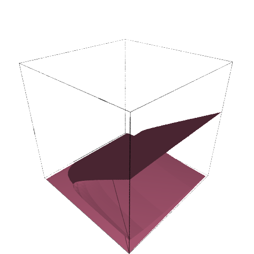
implicit_plot3d(f.diff(x),(k,0,25),(r,0.1,0.7),(x,0,20),color='palevioletred').show(viewer='tachyon')

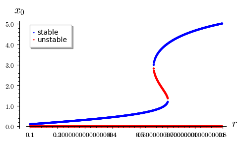
Problem 3: stability of stationary states

k_ = 6.6
x_stab = []
x_unstab = []
for r_ in srange(0.1,0.8,0.001):
    for x0 in get_n_roots(r_,k_)[1]:
        if f.diff(x).subs({k:k_,r:r_})(x0)<0:
            x_stab.append( (r_, x0) )
        else:
            x_unstab.append( (r_, x0) )

p = point(x_stab, legend_label='stable')
p += point(x_unstab,color='red', legend_label='unstable')
p.show(axes_labels=[r'$r$',r'$x_0$'], tick_formatter='latex', figsize=(5,3))

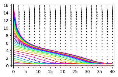
Time evolution

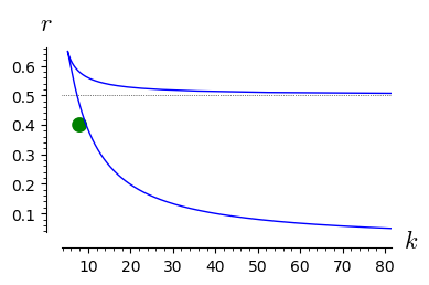
double_roots=line( [ (kx(x=x),rx(x=x)) for x in srange(1.01,42,0.01)],axes_labels=['$k$','$r$'],gridlines=[None,[0.5]],figsize=4 )
var('x')
for r_,k_ in [(0.4,12),(0.4,8)]:
    rk=point((k_,r_),size=100,color='green',xmax=80)

    t = var('t');
    x = function('x')(t)
    DE = diff(x, t) == f.subs({k:k_,r:r_})(x)
    g = []
    for i in srange(0, 16, .5):
        g.append ( line(desolve_rk4(DE, x, ics=[0, i], step=1.5, end_points=[40]),hue=sqrt(i) ) )

    x = var('x')
    g.append( plot_vector_field( (1,f.subs({k:k_,r:r_})(x) ) , (t, 0, 40), (x, 0, 16),figsize=4) )

    show(r"$r=%02f\; k=%02f$" % (r_,k_))
    show(sum(g))
    show(rk+double_roots)

$$\newcommand{\Bold}[1]{\mathbf{#1}}\verb|$r=0.400000\;|\phantom{\verb!x!}\verb|k=12.000000$|$$ $$\newcommand{\Bold}[1]{\mathbf{#1}}\verb|$r=0.400000\;|\phantom{\verb!x!}\verb|k=8.000000$|$$

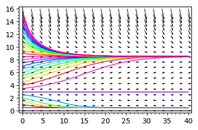
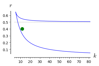
From the above analysis it follows the following:

1. The parameter space is devided into two parts: one where there is only one stable stationary state and one where there are two stable stationary states and one unstable state (not realizable).

2. In the regime when only one stable state is realized, for any initial conditions the system tends to this state.

3. In the regime of two coexisting stable stationary states, the initial condition are crucial. In dependence of its value, the system can tend to the state of smaller or greater value.

4. In the case of population of animals, the state of greater value is expected. In the case of tumor cells, the state of smaller value is desired.

5. It allows to develop strategy how to proceed.

We should keep some distance with respect to application of models. In the subject considered, although much progress has been made building mathematical models of tumor growth, they have not been centered on clinical data. Consequently, these models have had limited impact on clinical practice. It is not enough to test the effect of various assumptions mathematically (in silico); if they are to be of clinical value, these models must make predictions based on data that can be readily measured in people and that can be readily tested (falsified) in the clinic.